GuidingCenter · Stellarator particle orbits
Guiding-center orbits in a GVEC stellarator
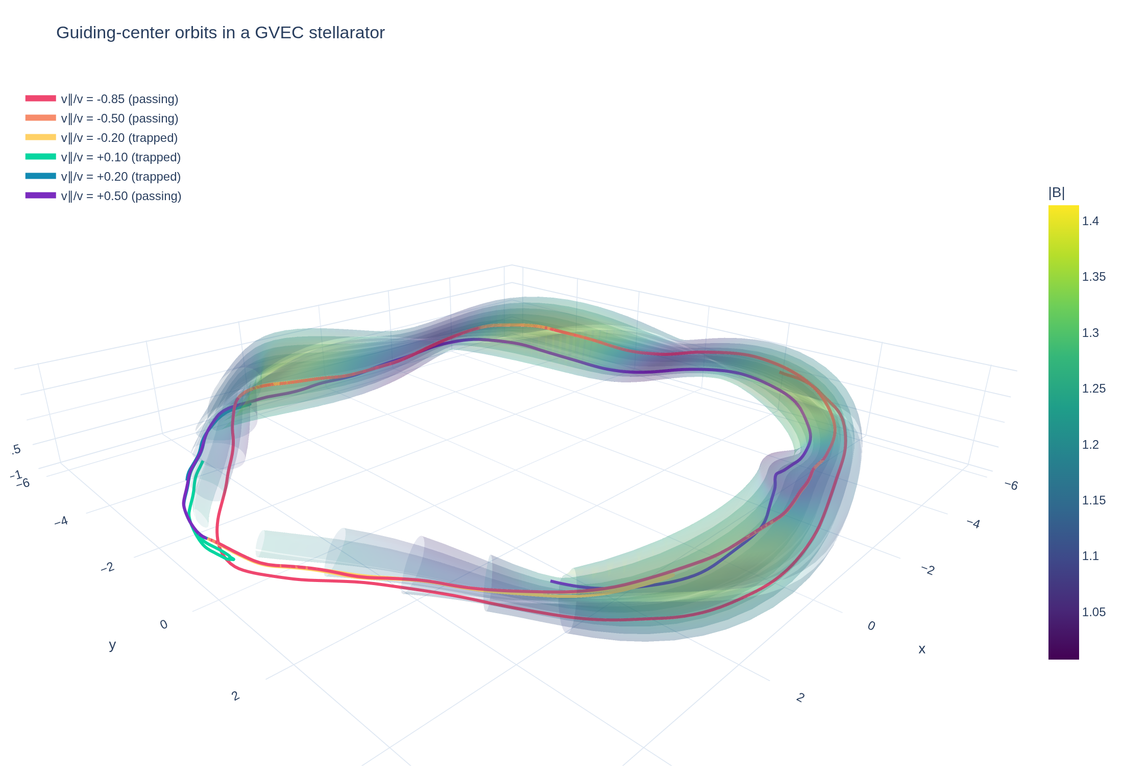
GVEC creates a five-field-period stellarator equilibrium, then Struphy follows passing and mirror-trapped guiding centers in its three-dimensional magnetic field.


Physical problem
Guiding centers in a generated GVEC stellarator
GVEC creates a five-field-period stellarator equilibrium, then Struphy follows passing and mirror-trapped guiding centers in its three-dimensional magnetic field.
PDEs solved by model:
Guiding-center Vlasov equation:
where is the guiding center distribution and
Simulation geometry
Domain used in this run
The actual GVECunit geometry reconstructed from this run's metadata. Switch between the 3D view and physical-coordinate slices.
Domain
GVECunit
Mapping
Loading GVECunit…
Parameters
| Parameter | Value | Description |
|---|---|---|
| Loading parameters… | ||
- Model
- GuidingCenter
- Grid
- 8 × 16 × 16
- FEEC degree
- 2 × 2 × 2
- Integrator
- Discrete gradient 1st order
- Evolution
- 2,000 steps
- Visualization
- Plotly
Performance
Profiling
Struphy's built-in scope-profiler instruments every propagator, pusher and solver call — these are the real per-call timings from the run above.
Durations
Gantt (rank 0)
Region statistics
| Region | Count | Avg (s) | Min (s) | Max (s) | Total (s) |
|---|
Complete source
Simulation script
Requires Struphy with compiled kernels and Plotly. Run struphy compile once, then execute python gvec-equilibrium.py.
"""Create a compact GVEC MHD equilibrium, then use it as a Struphy magnetic geometry.

GVEC first minimizes a five-field-period stellarator equilibrium defined entirely by
a Python parameter dictionary. Its newly written final state is passed directly to Struphy's `GVECequilibrium`,
which supplies both the curved `GVECunit` mapping and the equilibrium magnetic
field to Struphy's guiding-center model. The figures expose the resulting
three-dimensional flux geometry and particle orbits, one panel per marker with its
orbit projected on the poloidal plane, a poloidal cut with the radial equilibrium
profiles, and orbit diagnostics from the Struphy run.

The grid covers a single field period, which is what lets it resolve the helical
magnetic wells: markers launched with a small parallel velocity are mirror-trapped
in them, the faster ones circulate.

Requires the optional physics dependencies (`pip install -e ".[phys]"`) and
compiled Struphy kernels (`struphy compile`).
"""

from pathlib import Path
from types import MethodType

import h5py
import numpy as np
import plotly.graph_objects as go

from struphy import (
    BoundaryParameters,
    DerhamOptions,
    EnvironmentOptions,
    LoadingParameters,
    SavingParameters,
    Simulation,
    Time,
    WeightsParameters,
    domains,
    equils,
    grids,
    maxwellians,
)
from struphy.models import GuidingCenter

# Keep both the GVEC solve and the following FEEC simulation deliberately
# small. The complete equilibrium input is defined below, so the example has
# no external parameter or state-file dependency.
# The grid covers one field period (`use_nfp=True`), so its ten-ish toroidal elements resolve a single
# helical ripple. Spanning the whole torus instead would put two elements on each of the five ripples,
# which smooths away the magnetic wells and leaves every orbit passing.
mapping_elements = (8, 16, 16)
mapping_degree = (2, 2, 2)
speed = 1.5
pitches = (-0.85, -0.5, -0.2, 0.1, 0.2, 0.5)
start_rho = 0.55


grad_b_step = 1e-5  # central-difference step in logical coordinates


def gvec_grad_b_1(equilibrium, *etas, squeeze_out=False):
    """Covariant derivatives of |B| in Struphy's logical coordinates, by central differences.

    `GuidingCenter` needs ∇|B|, which Struphy's GVEC adapter does not provide
    (`GVECequilibrium.gradB1` raises `NotImplementedError`). GVEC exposes exact derivatives with
    respect to its own (r, θ, ζ), but Struphy's logical cube is not a per-axis rescaling of those
    coordinates, so converting them needs the full Jacobian of the map rather than three factors.
    Differencing `absB0` instead is consistent by construction with the field strength the model
    evaluates, at the cost of six evaluations per call — negligible for a handful of markers.

    The first direction is radial and not periodic, so samples are kept inside the domain and the
    true spacing is used; the two angles wrap around. Only grid evaluation is supported, which is how
    the equilibrium is consumed: `Propagator.projected_equil` projects ∇|B| onto the FEEC spaces once,
    and `GVECequilibrium.absB0` does not support flat marker evaluation either.
    """
    if len(etas) != 3:
        raise NotImplementedError("gvec_grad_b_1 evaluates on a grid; pass eta1, eta2, eta3")
    coordinates = [np.atleast_1d(np.asarray(eta, dtype=float)) for eta in etas]

    derivatives = []
    for axis in range(3):
        upper = coordinates[axis] + grad_b_step
        lower = coordinates[axis] - grad_b_step
        if axis == 0:
            upper = np.minimum(upper, 1.0)
            lower = np.maximum(lower, 0.0)
            spacing = upper - lower  # one-sided at the radial boundaries
        else:
            upper = np.mod(upper, 1.0)
            lower = np.mod(lower, 1.0)
            spacing = 2.0 * grad_b_step

        def sample(shifted):
            shifted_coordinates = list(coordinates)
            shifted_coordinates[axis] = shifted
            return equilibrium.absB0(*shifted_coordinates, squeeze_out=squeeze_out)

        derivatives.append((sample(upper) - sample(lower)) / spacing)
    return tuple(derivatives)


def gvec_parameters() -> dict:
    """A complete five-field-period stellarator equilibrium defined through pyGVEC's API."""
    return {
        "ProjectName": "struphy_gallery_stellarator",
        "whichInitEquilibrium": 0,
        "init_LA": True,
        "iota": {"type": "polynomial", "scale": -1.0, "coefs": (0.86, -0.08)},
        "pres": {"type": "polynomial", "scale": 1.0, "coefs": (0.02, -0.0137)},
        "PsiEdge": 1.0,
        # A compact, reduced stellarator boundary. Non-zero toroidal Fourier
        # modes twist both the magnetic axis and the last closed flux surface
        # through five field periods; no external input or state file is used.
        "X1_b_cos": {
            (0, 0): 5.5,
            (0, 1): 0.2354,
            (1, -1): -0.2233,
            (1, 0): 0.47685,
            (1, 1): -0.0121,
            (2, -1): 0.1,
            (2, 0): 0.0616,
        },
        "X2_b_sin": {
            (0, 1): 0.1155,
            (1, -1): 0.2233,
            (1, 0): 0.62315,
            (1, 1): -0.0121,
            (2, -1): 0.132,
            (2, 0): 0.06435,
        },
        "X1_a_cos": {(0, 0): 5.59625, (0, 1): 0.3586},
        "X2_a_sin": {(0, 1): 0.28765},
        "sgrid": {"nElems": 5, "grid_type": 0},
        "degGP": 8,
        "X1X2_deg": 5,
        "LA_deg": 5,
        "X1_mn_max": (2, 2),
        "X2_mn_max": (2, 2),
        "LA_mn_max": (2, 2),
        "X1_sin_cos": "_cos_",
        "X2_sin_cos": "_sin_",
        "LA_sin_cos": "_sin_",
        "nfp": 5,
        "start_dt": 0.3,
        "PrecondType": 1,
        "MinimizerType": 10,
        "maxiter": 1000,
        "totaliter": 1000,
        "minimize_tol": 1.0e-4,
    }


def create_gvec_equilibrium(workdir: Path) -> tuple[equils.GVECequilibrium, int, float]:
    """Run GVEC from our Python parameters and expose its new final state to Struphy."""
    import gvec

    # pyGVEC writes our new parameter and state files into `workdir`. This
    # compact case normally converges in fewer than five hundred iterations.
    run = gvec.run(
        gvec_parameters(), runpath=workdir, quiet=True, redirect_gvec_stdout=True
    )
    equilibrium = equils.GVECequilibrium(
        rel_path=False,
        param_file=str(run.state.parameterfile),
        dat_file=str(run.state.statefile),
        use_nfp=True,
        num_elements=mapping_elements,
        degree=mapping_degree,
    )
    equilibrium.gradB1 = MethodType(gvec_grad_b_1, equilibrium)
    return equilibrium, int(run.GVEC_iter_used), float(run.max_force)


def make_simulation(equilibrium, folder: str, domain=None, **extra) -> Simulation:
    simulation_domain = domain or equilibrium.numerical_domain
    if domain is not None:
        equilibrium.domain = simulation_domain
    b_start = float(equilibrium.absB0(start_rho, 0.0, 0.0, squeeze_out=True))
    initial = tuple(
        (
            start_rho,
            0.0,
            0.0,
            speed * pitch,
            speed**2 * (1.0 - pitch**2) / (2.0 * b_start),
        )
        for pitch in pitches
    )
    model = GuidingCenter()
    model.kinetic_ions.set_markers(
        loading_params=LoadingParameters(
            Np=len(initial), seed=1, specific_markers=initial
        ),
        weights_params=WeightsParameters(),
        boundary_params=BoundaryParameters(bc=("remove", "periodic", "periodic")),
        saving_params=SavingParameters(n_markers=1.0),
        bufsize=2.0,
    )
    model.propagators.push_bxe.options = model.propagators.push_bxe.Options(
        maxiter=100, tol=1e-8
    )
    model.propagators.push_parallel.options = model.propagators.push_parallel.Options(
        maxiter=100, tol=1e-8
    )
    model.kinetic_ions.var.add_background(
        maxwellians.GyroMaxwellian2D(n=(1.0, None), B0=b_start)
    )
    return Simulation(
        model=model,
        env=EnvironmentOptions(
            out_folders="struphy_gallery_runs", sim_folder=folder, save_step=5
        ),
        time_opts=Time(dt=0.02, Tend=40.0, split_algo="Strang"),
        domain=simulation_domain,
        equil=equilibrium,
        grid=grids.TensorProductGrid(num_elements=mapping_elements),
        derham_opts=DerhamOptions(
            degree=mapping_degree, bcs=(("free", "free"), None, None)
        ),
        **extra,
    )


# Metadata generation imports this script without executing GVEC. The cheap
# placeholder below is never run; `metadata_overrides` records the runtime
# geometry, while the executable block replaces it with our generated state.
simulation_details = {
    "name": "Guiding-center orbits in a GVEC stellarator",
    "description": (
        "GVEC creates a five-field-period stellarator equilibrium, then Struphy follows passing and "
        "mirror-trapped guiding centers in its three-dimensional magnetic field."
    ),
}
sim = make_simulation(
    equils.HomogenSlab(B0z=1.0),
    "gvec_equilibrium_metadata",
    domain=domains.Cuboid(),
    **simulation_details,
)
metadata_overrides = {"domain": "GVECunit (generated by pyGVEC)"}


if __name__ == "__main__":
    from plotly.subplots import make_subplots

    from _gallery import (
        export_profiling,
        merge_metadata,
        save_extra_figure,
        save_figure,
    )

    gvec_directory = Path("struphy_gallery_runs/gvec_equilibrium_source")
    gvec_directory.parent.mkdir(parents=True, exist_ok=True)
    equilibrium, gvec_iterations, gvec_force = create_gvec_equilibrium(gvec_directory)
    run = make_simulation(
        equilibrium, "gvec_equilibrium", name=sim.name, description=sim.description
    )
    run.run(profiling_activated=True)

    # Keep the live GVEC mapping for post-processing. A GVECunit reconstructed
    # only from generic run metadata does not retain its generated state file.
    data_file = Path(run.env.path_out) / "data/data_proc0.hdf5"
    with h5py.File(data_file) as data:
        time = np.asarray(data["time/value"])
        saved_markers = np.asarray(data["kinetic/kinetic_ions/markers"])
        total_energy = np.asarray(data["scalar/en_tot"])
        lost_history = np.asarray(data["scalar/n_lost_particles"])
    marker_history = np.empty((len(time), len(pitches), saved_markers.shape[-1]))
    for step, marker_rows in enumerate(saved_markers):
        active = marker_rows[marker_rows[:, -1] >= 0]
        if len(active) != len(pitches):
            raise RuntimeError("A guiding center left the GVEC radial domain")
        marker_history[step] = active[np.argsort(active[:, -1])]
    logical_positions = marker_history[:, :, :3]
    physical_positions = equilibrium.numerical_domain(
        logical_positions.reshape(-1, 3), change_out_order=True
    ).reshape(logical_positions.shape)
    x, y, z = np.moveaxis(physical_positions, -1, 0)

    # The grid holds one field period, so a marker that leaves it re-enters at the other end and comes
    # back mapped into the same wedge: its toroidal angle jumps by 2*pi/nfp. Unwrapping that angle and
    # rebuilding the position from (R, phi, Z) continues each orbit into the next period, which the
    # equilibrium's field-period symmetry makes exact.
    field_periods = int(equilibrium.state.nfp)
    major_radius = np.hypot(x, y)
    toroidal_angle = np.unwrap(np.arctan2(y, x), period=2.0 * np.pi / field_periods, axis=0)
    x, y = major_radius * np.cos(toroidal_angle), major_radius * np.sin(toroidal_angle)
    v_parallel = marker_history[:, :, 3]
    reflections = np.array(
        [
            np.count_nonzero(np.diff(np.sign(column[np.isfinite(column)])))
            for column in v_parallel.T
        ]
    )
    reflected = reflections > 0
    labels = [
        f"v∥/v = {pitch:+.2f} ({'trapped' if reflected[index] else 'passing'})"
        for index, pitch in enumerate(pitches)
    ]
    colors = ("#ef476f", "#f78c6b", "#ffd166", "#06d6a0", "#118ab2", "#7b2cbf")

    relative_energy = np.abs(total_energy / total_energy[0] - 1.0)
    relative_drift = float(np.nanmax(relative_energy))
    lost_markers = int(np.nanmax(lost_history))
    if not np.isfinite(relative_drift):
        raise RuntimeError(
            "Non-finite energy diagnostic in the GVEC guiding-center run"
        )
    print(
        f"GVEC converged in {gvec_iterations} iterations to |force| = {gvec_force:.2e}; "
        f"field periods: {equilibrium.state.nfp}; reflections per orbit: {reflections.tolist()}; "
        f"guiding-center energy drift: {relative_drift:.2e}"
    )

    # A cutaway stellarator makes the nested GVEC flux surfaces visible behind
    # the guiding-center trajectories. Surface color is the magnetic strength.
    surface_radii = np.array((0.2, 0.4, 0.6, 0.8, 1.0))
    toroidal_angles = np.linspace(0.05 * np.pi, 1.95 * np.pi, 97)
    surface_data = equilibrium.state.evaluate(
        "pos",
        "mod_B",
        rho=surface_radii,
        theta=49,
        zeta=toroidal_angles,
    )
    positions = np.asarray(surface_data["pos"])
    field_strength = np.asarray(surface_data["mod_B"])
    field_min = float(np.nanmin(field_strength))
    field_max = float(np.nanmax(field_strength))

    figure = go.Figure()
    for index, radius in enumerate(surface_radii):
        # Trim progressively more toroidal sections from the larger shells.
        # The staggered cut exposes every nested surface in the open wedge.
        trim = 3 * index
        toroidal_slice = slice(trim, len(toroidal_angles) - trim)
        figure.add_trace(
            go.Surface(
                x=positions[0, index, :, toroidal_slice],
                y=positions[1, index, :, toroidal_slice],
                z=positions[2, index, :, toroidal_slice],
                surfacecolor=field_strength[index, :, toroidal_slice],
                cmin=field_min,
                cmax=field_max,
                colorscale="Viridis",
                opacity=0.10 + 0.02 * index,
                showscale=index == len(surface_radii) - 1,
                colorbar={"title": "|B|", "len": 0.72},
                name=f"ρ = {radius:.1f}",
                hovertemplate=(
                    f"ρ = {radius:.1f}<br>R = %{{customdata:.3f}}<br>"
                    "Z = %{z:.3f}<br>|B| = %{surfacecolor:.3f}<extra></extra>"
                ),
                customdata=np.sqrt(
                    positions[0, index, :, toroidal_slice] ** 2
                    + positions[1, index, :, toroidal_slice] ** 2
                ),
            )
        )
    for index, label in enumerate(labels):
        figure.add_trace(
            go.Scatter3d(
                x=x[:, index],
                y=y[:, index],
                z=z[:, index],
                mode="lines",
                line={"color": colors[index], "width": 6},
                name=label,
                hovertemplate=(
                    f"{label}<br>x = %{{x:.3f}}<br>y = %{{y:.3f}}<br>"
                    "z = %{z:.3f}<extra></extra>"
                ),
            )
        )
    figure.update_layout(
        title="Guiding-center orbits in a GVEC stellarator",
        template="plotly_white",
        scene={
            "xaxis_title": "x",
            "yaxis_title": "y",
            "zaxis_title": "z",
            "aspectmode": "data",
            "camera": {"eye": {"x": 1.45, "y": 1.45, "z": 0.85}},
        },
        legend={"x": 0.01, "y": 0.99, "bgcolor": "rgba(255,255,255,0.72)"},
        margin={"l": 10, "r": 30, "t": 75, "b": 10},
    )
    save_figure(figure, "gvec-equilibrium", height=760)

    # A poloidal slice reveals the nesting more quantitatively; the adjacent
    # radial profiles come from the very same state file used by Struphy.
    cut_radii = np.linspace(0.1, 1.0, 10)
    # The cut at zeta = 0 for the flux-surface panel, and a few more across one field period: the
    # cross-section of a stellarator turns with the toroidal angle, so a projected orbit lives inside
    # the envelope of all of them rather than on any single cut.
    panel_angles = np.linspace(0.0, 2.0 * np.pi / int(equilibrium.state.nfp), 5)
    cut_data = equilibrium.state.evaluate(
        "pos", rho=cut_radii, theta=181, zeta=np.append(np.array((0.0,)), panel_angles)
    )
    cut_positions = np.asarray(cut_data["pos"])[..., :1]
    panel_positions = np.asarray(cut_data["pos"])[..., 1:]
    profile_radii = np.linspace(0.0, 1.0, 101)
    profile_data = equilibrium.state.evaluate(
        "iota", "p", rho=profile_radii, theta=0, zeta=0
    )

    profiles = make_subplots(
        rows=1,
        cols=2,
        specs=[[{}, {"secondary_y": True}]],
        subplot_titles=(
            "Poloidal flux surfaces (ζ = 0)",
            "Radial equilibrium profiles",
        ),
        horizontal_spacing=0.14,
    )
    for index, radius in enumerate(cut_radii):
        # Not x, y, z: those hold the orbits, which the panels below still need.
        cut_x = cut_positions[0, index, :, 0]
        cut_y = cut_positions[1, index, :, 0]
        cut_z = cut_positions[2, index, :, 0]
        radial_position = np.sqrt(cut_x**2 + cut_y**2)
        profiles.add_scatter(
            x=np.append(radial_position, radial_position[0]),
            y=np.append(cut_z, cut_z[0]),
            mode="lines",
            line={"color": "#168aad", "width": 1.5 + 1.2 * radius},
            opacity=0.35 + 0.65 * radius,
            name=f"ρ = {radius:.1f}",
            legendgroup="surfaces",
            showlegend=index in (0, len(cut_radii) - 1),
            row=1,
            col=1,
        )
    profiles.add_scatter(
        x=profile_radii,
        y=np.asarray(profile_data["p"]),
        mode="lines",
        name="pressure p",
        line={"color": "#d62828", "width": 3},
        row=1,
        col=2,
        secondary_y=False,
    )
    profiles.add_scatter(
        x=profile_radii,
        y=np.asarray(profile_data["iota"]),
        mode="lines",
        name="rotational transform ι",
        line={"color": "#f4a261", "width": 3},
        row=1,
        col=2,
        secondary_y=True,
    )
    profiles.update_xaxes(title_text="R", scaleanchor="y", scaleratio=1, row=1, col=1)
    profiles.update_yaxes(title_text="Z", row=1, col=1)
    profiles.update_xaxes(title_text="normalized flux radius ρ", row=1, col=2)
    profiles.update_yaxes(title_text="pressure p", row=1, col=2, secondary_y=False)
    profiles.update_yaxes(
        title_text="rotational transform ι", row=1, col=2, secondary_y=True
    )
    profiles.update_layout(
        title="GVEC flux geometry and equilibrium profiles",
        template="plotly_white",
        legend={"orientation": "h", "y": -0.2},
        margin={"l": 70, "r": 70, "t": 90, "b": 100},
    )
    figures = [
        save_extra_figure(
            profiles,
            "gvec-equilibrium",
            "flux-surfaces",
            alt="Nested GVEC flux surfaces in a poloidal cut beside pressure and rotational-transform profiles",
            caption=(
                "A poloidal cut through the nested magnetic surfaces generated by GVEC. "
                "The pressure and rotational transform on the right are evaluated directly "
                "from the newly generated equilibrium state."
            ),
        )
    ]

    # One panel per marker, the orbit projected on the (R, Z) plane, as in the tokamak example. The
    # cross-section of a stellarator turns with the toroidal angle, so the surfaces drawn behind each
    # orbit are the cut at zeta = 0: context for the radial excursion, not a plane the orbit stays in.
    panels = make_subplots(
        rows=2,
        cols=3,
        subplot_titles=labels,
        horizontal_spacing=0.05,
        vertical_spacing=0.13,
    )
    panel_radial = np.sqrt(panel_positions[0] ** 2 + panel_positions[1] ** 2)
    panel_height = panel_positions[2]
    radius_range = [
        min(panel_radial.min(), major_radius.min()) - 0.1,
        max(panel_radial.max(), major_radius.max()) + 0.1,
    ]
    height_range = [
        min(panel_height.min(), z.min()) - 0.1,
        max(panel_height.max(), z.max()) + 0.1,
    ]
    for index, label in enumerate(labels):
        row, column = divmod(index, 3)
        for surface in range(len(cut_radii)):
            for angle in range(panel_radial.shape[-1]):
                panels.add_scatter(
                    x=np.append(panel_radial[surface, :, angle], panel_radial[surface, 0, angle]),
                    y=np.append(panel_height[surface, :, angle], panel_height[surface, 0, angle]),
                    mode="lines",
                    line={"color": "#b8c4cc", "width": 1},
                    opacity=0.35,
                    showlegend=False,
                    hoverinfo="skip",
                    row=row + 1,
                    col=column + 1,
                )
        panels.add_scatter(
            x=major_radius[:, index],
            y=z[:, index],
            mode="lines",
            line={"color": colors[index], "width": 2},
            showlegend=False,
            hovertemplate="R = %{x:.3f}<br>Z = %{y:.3f}<extra></extra>",
            row=row + 1,
            col=column + 1,
        )
        panels.add_scatter(
            x=[major_radius[0, index]],
            y=[z[0, index]],
            mode="markers",
            marker={"color": "#222", "size": 7, "symbol": "circle-open", "line": {"width": 2}},
            showlegend=False,
            hoverinfo="skip",
            row=row + 1,
            col=column + 1,
        )
        axis_index = index + 1
        panels.update_xaxes(
            title_text="R" if row == 1 else None, range=radius_range, row=row + 1, col=column + 1
        )
        panels.update_yaxes(
            title_text="Z" if column == 0 else None,
            range=height_range,
            scaleanchor="x" if axis_index == 1 else f"x{axis_index}",
            scaleratio=1,
            row=row + 1,
            col=column + 1,
        )
    panels.update_layout(
        title="Guiding-center orbits projected on the poloidal plane",
        template="plotly_white",
        margin={"l": 70, "r": 30, "t": 90, "b": 60},
        height=760,
    )
    figures.append(
        save_extra_figure(
            panels,
            "gvec-equilibrium",
            "poloidal-orbits",
            alt="One panel per marker showing its guiding-center orbit projected on the poloidal plane",
            caption=(
                "Each marker's orbit projected on the (R, Z) plane. The grey curves are the flux surfaces at "
                "five toroidal angles across one field period, whose envelope is the region the projection "
                "can reach. "
                "The trapped markers stay within a narrow band of flux surfaces and retrace it, while the "
                "passing ones sweep the whole cross-section as they circulate. Unlike a tokamak, the "
                "stellarator cross-section rotates with the toroidal angle, so these projections are not "
                "closed banana curves: the width of the band is the radial excursion, the filling-in is the "
                "toroidal motion."
            ),
        )
    )

    diagnostics = make_subplots(
        rows=1,
        cols=2,
        subplot_titles=("Parallel velocity", "Total guiding-center energy"),
        horizontal_spacing=0.13,
    )
    for index, label in enumerate(labels):
        diagnostics.add_scatter(
            x=time,
            y=v_parallel[:, index] / speed,
            mode="lines",
            name=label,
            line={"color": colors[index], "width": 2.2},
            row=1,
            col=1,
        )
    diagnostics.add_hline(y=0.0, line={"color": "#888", "width": 1}, row=1, col=1)
    diagnostics.add_scatter(
        x=time,
        y=np.maximum(relative_energy, 1.0e-14),
        mode="lines",
        name="relative energy change",
        line={"color": "#264653", "width": 3},
        row=1,
        col=2,
    )
    diagnostics.update_xaxes(title_text="t [a.u.]", row=1, col=1)
    diagnostics.update_xaxes(title_text="t [a.u.]", row=1, col=2)
    diagnostics.update_yaxes(title_text="v∥ / v", row=1, col=1)
    diagnostics.update_yaxes(
        title_text="|E / E₀ − 1|", type="log", exponentformat="power", row=1, col=2
    )
    diagnostics.update_layout(
        title="Orbit classification and conservation",
        template="plotly_white",
        legend={"orientation": "h", "y": -0.2},
        margin={"l": 75, "r": 30, "t": 80, "b": 100},
    )
    figures.append(
        save_extra_figure(
            diagnostics,
            "gvec-equilibrium",
            "orbit-diagnostics",
            alt="Parallel velocities and total-energy conservation of guiding-center orbits in the GVEC stellarator",
            caption=(
                "A sign change in parallel velocity identifies a magnetic-mirror reflection: the markers "
                "launched with a small parallel velocity are caught in the helical wells of the stellarator, "
                "while the faster ones circulate. The magnetic moment is a coordinate of the model and is "
                "conserved exactly; the total energy drifts by a few percent, which is set by the accuracy "
                "of the coarse FEEC projection of the GVEC field rather than by the time integrator — the "
                "drift does not fall when the time step is reduced."
            ),
        )
    )
    merge_metadata(
        "gvec-equilibrium",
        gvecIterations=gvec_iterations,
        gvecFinalForce=gvec_force,
        gvecFieldPeriods=int(equilibrium.state.nfp),
        markers=len(pitches),
        reflectedMarkers=int(reflected.sum()),
        lostMarkers=lost_markers,
        relativeEnergyDrift=relative_drift,
        figures=figures,
        **export_profiling(run, "gvec-equilibrium"),
    )
See the post-processing guide for more ways to inspect the result.