PressureLessSPH · Pressureless particle flow
SPH in a Beltrami force field
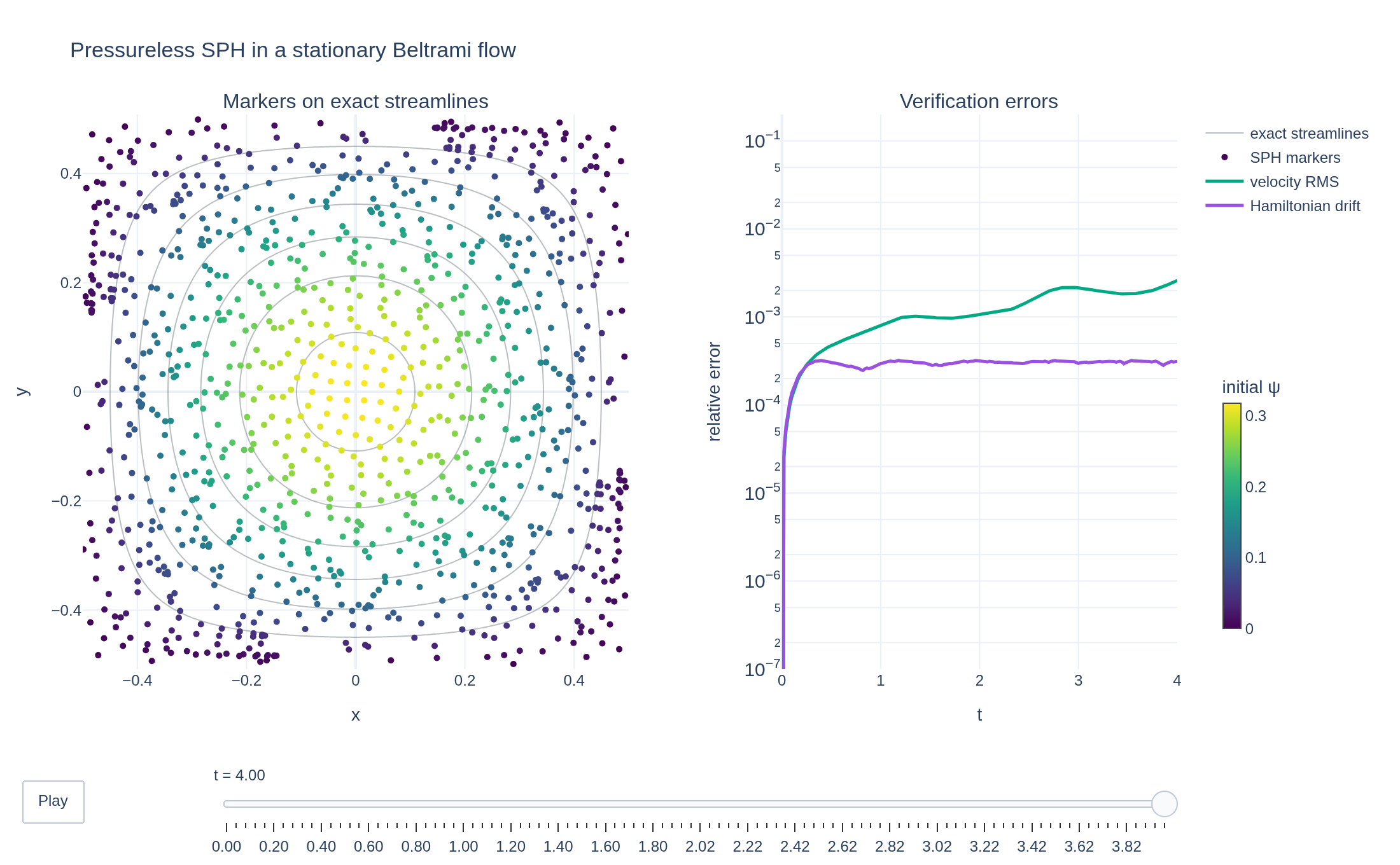
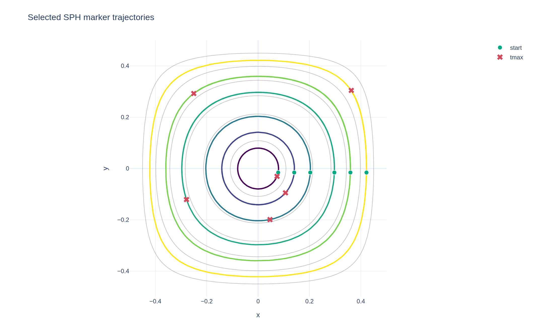
Pressureless SPH markers circulate through a stationary cellular flow driven by a prescribed Beltrami potential. The computed marker velocity is compared with the exact Eulerian velocity field, while conservation of each marker's kinetic-plus-potential energy checks the orbit integration.
Loading interactive figure…
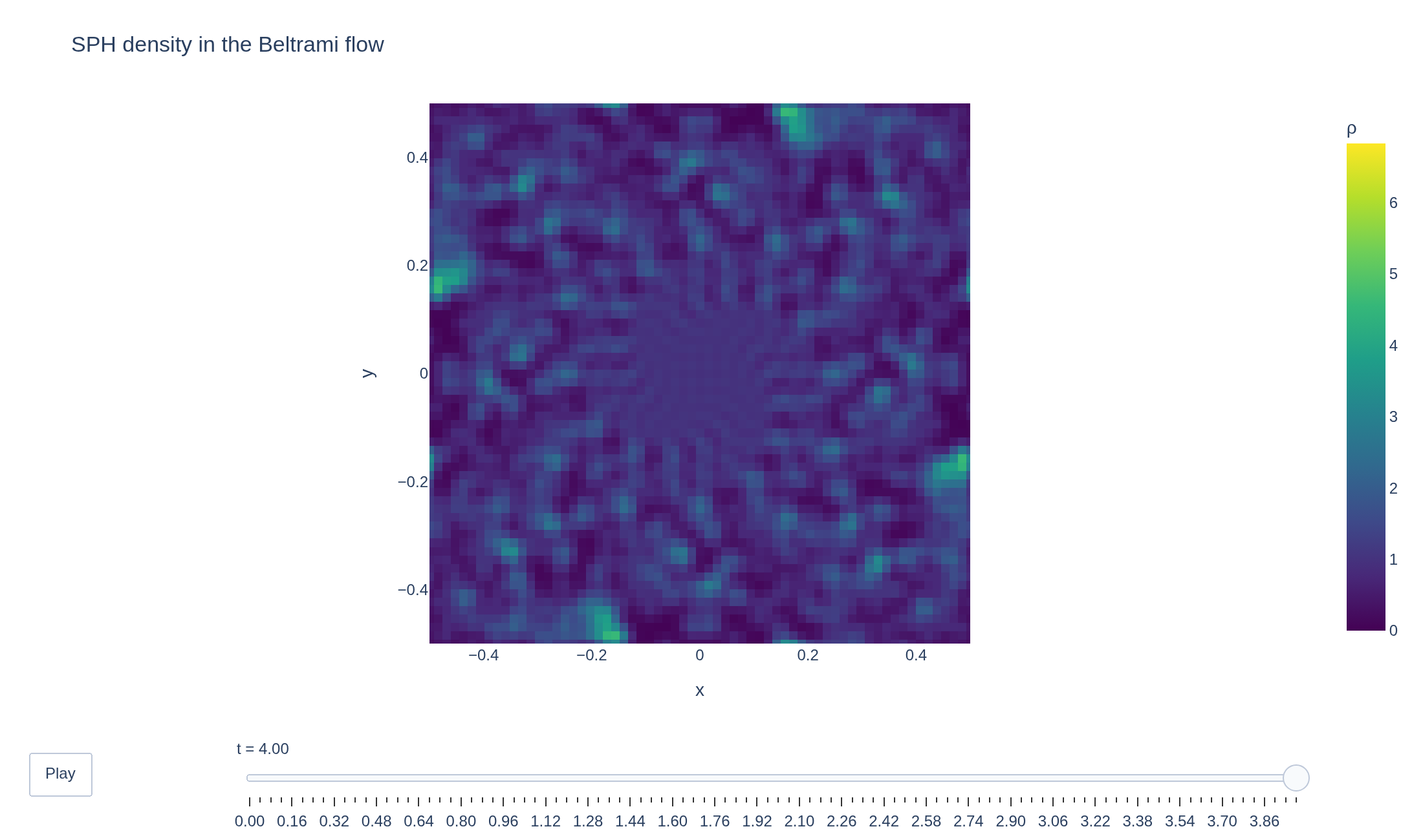
Loading interactive figure…
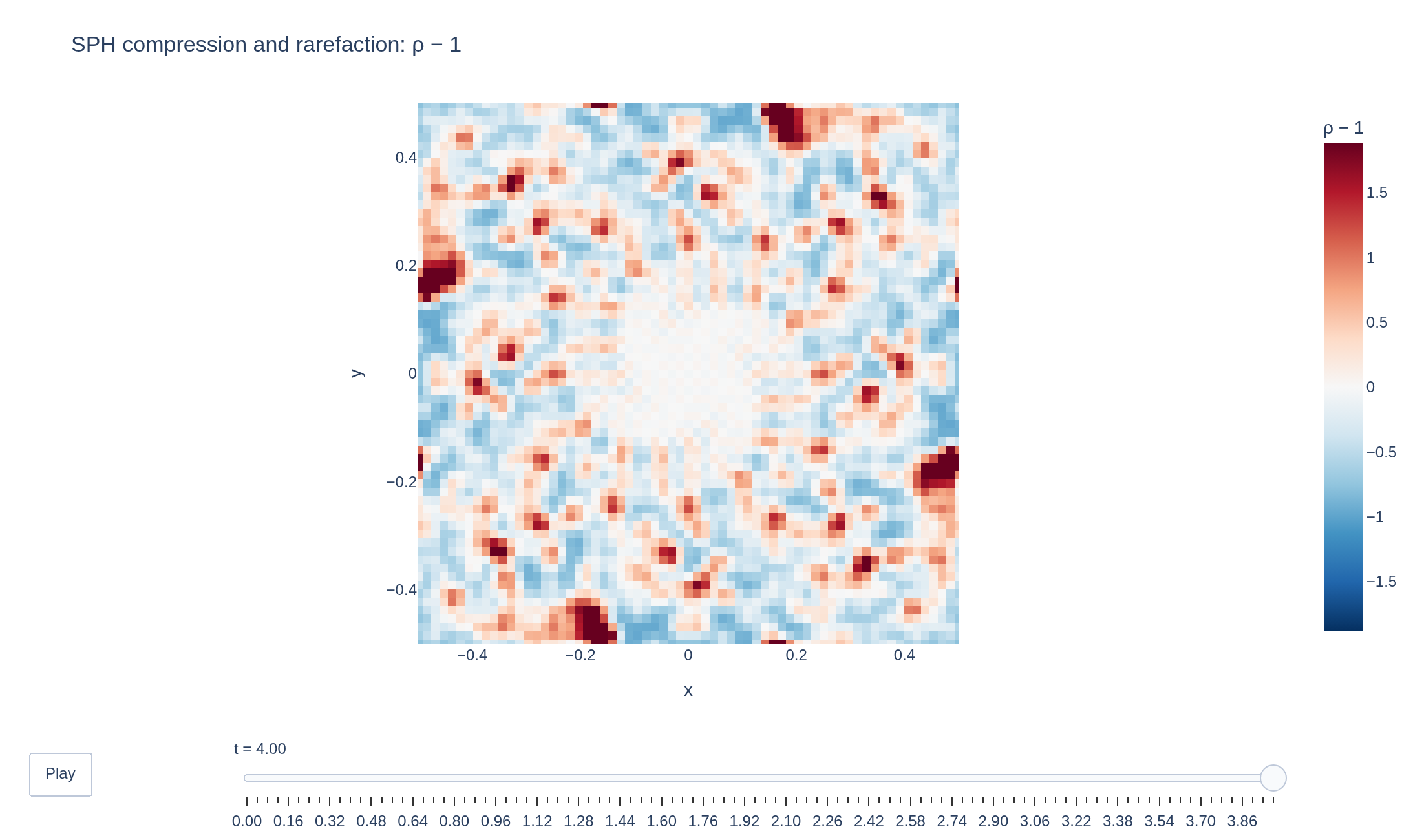
Loading interactive figure…
Loading interactive figure…
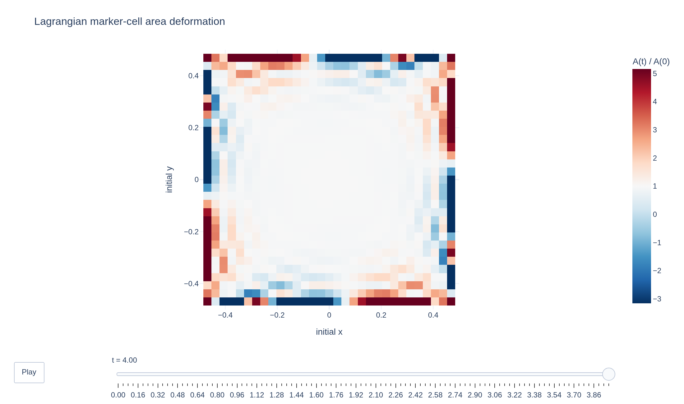
Loading interactive figure…
Physical problem
Markers following a stationary cellular flow
Pressureless SPH markers circulate through a stationary cellular flow driven by a prescribed Beltrami potential. The computed marker velocity is compared with the exact Eulerian velocity field, while conservation of each marker's kinetic-plus-potential energy checks the orbit integration.
Adapted from the corresponding Struphy tutorial.
PDEs solved by model:
Continuity:
Momentum:
where is an external force.
Simulation geometry
Domain used in this run
The actual Cuboid geometry reconstructed from this run's metadata. Switch between the 3D view and physical-coordinate slices.
Domain
Cuboid
Mapping
Loading Cuboid…
Parameters
| Parameter | Value | Description |
|---|---|---|
| Loading parameters… | ||
- Model
- PressureLessSPH
- Grid
- 32 × 32 × 1
- FEEC degree
- 3 × 3 × 1
- Evolution
- 200 steps
- Visualization
- Plotly
Performance
Profiling
Struphy's built-in scope-profiler instruments every propagator, pusher and solver call — these are the real per-call timings from the run above.
Durations
Gantt (rank 0)
Region statistics
| Region | Count | Avg (s) | Min (s) | Max (s) | Total (s) |
|---|
Complete source
Simulation script
Requires Struphy with compiled kernels and Plotly. Run struphy compile once, then execute python beltrami-sph.py.
"""Pressureless SPH markers orbiting in a stationary Beltrami force field.
The two-dimensional velocity
u = (-cos(pi x) sin(pi y), sin(pi x) cos(pi y))
is a stationary solution of the pressureless momentum equation when the external
potential is p = (sin(pi x)^2 + sin(pi y)^2) / 2, because (u . grad)u = -grad p.
Markers initialized with this velocity should therefore keep following the same
Eulerian velocity field. Their particle Hamiltonian |v|^2 / 2 + p is conserved as
well. The animation shows the marker motion on stream-function contours while the
second panel reports both numerical errors.
Adapted from Struphy's ``tutorial_beltrami_sph.ipynb`` tutorial.
Requires Struphy 3.3 with compiled kernels (`struphy compile`).
"""
import numpy as np
import plotly.graph_objects as go
from plotly.subplots import make_subplots
from struphy import (
BoundaryParameters,
DerhamOptions,
EnvironmentOptions,
KernelDensityPlot,
LoadingParameters,
SavingParameters,
Simulation,
SortingParameters,
Time,
WeightsParameters,
domains,
equils,
grids,
)
from struphy.models import PressureLessSPH
from struphy.ode.utils import ButcherTableau
box_min = -0.5
box_max = 0.5
boxes = 16
markers_per_box = 4
density_points = 65
def velocity(x, y, z):
"""Stationary cellular-flow velocity in physical coordinates."""
del z
return (
-np.cos(np.pi * x) * np.sin(np.pi * y),
np.sin(np.pi * x) * np.cos(np.pi * y),
np.zeros_like(x),
)
def potential(x, y, z):
"""Potential whose negative gradient accelerates the stationary flow."""
del z
return 0.5 * (np.sin(np.pi * x) ** 2 + np.sin(np.pi * y) ** 2)
def density(x, y, z):
"""Uniform initial density."""
del y, z
return np.ones_like(x)
beltrami_flow = equils.GenericCartesianFluidEquilibrium(
u_xyz=velocity,
p_xyz=potential,
n_xyz=density,
)
model = PressureLessSPH(epsilon=1.0)
model.propagators.push_eta.options = model.propagators.push_eta.Options(
butcher=ButcherTableau(algo="forward_euler"),
)
model.propagators.push_v.potential = beltrami_flow.p0
model.cold_fluid.set_markers(
loading_params=LoadingParameters(ppb=markers_per_box, loading="tesselation"),
weights_params=WeightsParameters(),
boundary_params=BoundaryParameters(bc=("reflect", "reflect", "periodic")),
sorting_params=SortingParameters(
boxes_per_dim=(boxes, boxes, 1),
dims_mask=(True, True, False),
),
saving_params=SavingParameters(
n_markers=1.0,
kernel_density_plots=(
KernelDensityPlot(
pts_e1=density_points,
pts_e2=density_points,
pts_e3=1,
),
),
),
bufsize=0.5,
)
model.cold_fluid.var.add_background(beltrami_flow)
domain = domains.Cuboid(
l1=box_min,
r1=box_max,
l2=box_min,
r2=box_max,
l3=0.0,
r3=1.0,
)
env = EnvironmentOptions(
out_folders="struphy_gallery_runs",
sim_folder="beltrami_sph",
)
sim = Simulation(
model=model,
name="SPH in a Beltrami force field",
description=(
"Pressureless SPH markers circulate through a stationary cellular flow driven by a prescribed "
"Beltrami potential. The computed marker velocity is compared with the exact Eulerian velocity "
"field, while conservation of each marker's kinetic-plus-potential energy checks the orbit integration."
),
env=env,
time_opts=Time(dt=0.02, Tend=4.0, split_algo="Strang"),
domain=domain,
grid=grids.TensorProductGrid(num_elements=(32, 32, 1)),
derham_opts=DerhamOptions(
degree=(3, 3, 1),
bcs=(("free", "free"), ("free", "free"), None),
),
)
if __name__ == "__main__":
from _gallery import export_profiling, is_root, merge_metadata, save_extra_figure, save_figure
output = sim.run(profiling_activated=True)
output.pproc()
orbits = output.evaluate("cold_fluid")
rho = output.evaluate("cold_fluid/view_0/n").isel(e3=0)
times = np.asarray(orbits.t.values)
x, y, z = (np.asarray(orbits.sel(quantity=name).values) for name in ("x", "y", "z"))
v1, v2, v3 = (np.asarray(orbits.sel(quantity=name).values) for name in ("v1", "v2", "v3"))
values = np.stack((x, y, z, v1, v2, v3), axis=-1)
rho_values = np.asarray(rho.transpose("t", "e2", "e1").values)
if not (np.isfinite(values).all() and np.isfinite(rho_values).all()):
raise RuntimeError("Non-finite Beltrami result: refusing to publish the run")
if not np.isclose(times[-1], sim.time_opts.Tend):
raise RuntimeError(f"Incomplete Beltrami run: stopped at t={times[-1]:g}")
if not np.allclose(times, rho.t.values):
raise RuntimeError("Marker and density output times do not match")
exact_v1, exact_v2, _ = velocity(x, y, z)
initial_speed_rms = float(np.sqrt(np.mean(v1[0] ** 2 + v2[0] ** 2)))
velocity_error = np.sqrt(np.mean((v1 - exact_v1) ** 2 + (v2 - exact_v2) ** 2, axis=1))
velocity_error /= initial_speed_rms
hamiltonian = 0.5 * (v1**2 + v2**2 + v3**2) + potential(x, y, z)
hamiltonian_scale = np.maximum(np.abs(hamiltonian[0]), 1e-14)
energy_error = np.max(np.abs(hamiltonian - hamiltonian[0]) / hamiltonian_scale, axis=1)
max_velocity_error = float(np.max(velocity_error))
max_energy_error = float(np.max(energy_error))
if max_velocity_error > 0.1 or max_energy_error > 0.1:
raise RuntimeError(
"Beltrami verification failed: "
f"{max_velocity_error=:.3g}, {max_energy_error=:.3g}"
)
if is_root():
print(
f"maximum relative velocity RMS error {max_velocity_error:.3e}; "
f"maximum per-marker Hamiltonian drift {max_energy_error:.3e}"
)
# The stream function psi has u = (d_y psi, -d_x psi); its contours are exact trajectories.
mesh = np.linspace(box_min, box_max, 161)
mesh_x, mesh_y = np.meshgrid(mesh, mesh)
stream_function = np.cos(np.pi * mesh_x) * np.cos(np.pi * mesh_y) / np.pi
marker_color = np.cos(np.pi * x[0]) * np.cos(np.pi * y[0]) / np.pi
color_limit = float(np.max(np.abs(marker_color)))
def marker_trace(index):
return go.Scatter(
x=x[index],
y=y[index],
mode="markers",
name="SPH markers",
marker={
"size": 5,
"color": marker_color,
"colorscale": "Viridis",
"cmin": 0.0,
"cmax": color_limit,
"line": {"width": 0},
"colorbar": {
"title": "initial ψ",
"x": 1.03,
"xanchor": "left",
"y": 0.3,
"yanchor": "middle",
"len": 0.5,
"thickness": 14,
},
},
hovertemplate="x=%{x:.3f}<br>y=%{y:.3f}<extra></extra>",
)
contour = go.Contour(
x=mesh,
y=mesh,
z=stream_function,
contours={"coloring": "none", "showlabels": False},
line={"color": "rgba(40,55,65,.32)", "width": 1},
showscale=False,
hoverinfo="skip",
name="exact streamlines",
)
def error_trace(index, values, name, color):
"""Error history up to one animation frame."""
return go.Scatter(
x=times[: index + 1],
y=np.maximum(values[: index + 1], 1e-16),
xaxis="x2",
yaxis="y2",
mode="lines",
name=name,
line={"color": color, "width": 2.5},
)
figure = make_subplots(
rows=1,
cols=2,
column_widths=(0.58, 0.42),
horizontal_spacing=0.14,
subplot_titles=("Markers on exact streamlines", "Verification errors"),
)
figure.add_trace(contour, row=1, col=1)
figure.add_trace(marker_trace(0), row=1, col=1)
figure.add_trace(error_trace(0, velocity_error, "velocity RMS", "#00a884"), row=1, col=2)
figure.add_trace(error_trace(0, energy_error, "Hamiltonian drift", "#9b51e0"), row=1, col=2)
picks = np.unique(np.linspace(0, len(times) - 1, min(100, len(times)), dtype=int))
figure.frames = [
go.Frame(
name=f"{times[index]:.2f}",
data=[
marker_trace(index),
error_trace(index, velocity_error, "velocity RMS", "#00a884"),
error_trace(index, energy_error, "Hamiltonian drift", "#9b51e0"),
],
traces=[1, 2, 3],
)
for index in picks
]
figure.update_layout(
title="Pressureless SPH in a stationary Beltrami flow",
template="plotly_white",
margin={"l": 65, "r": 175, "t": 90, "b": 135},
legend={
"orientation": "v",
"x": 1.02,
"xanchor": "left",
"y": 1,
"yanchor": "top",
},
updatemenus=[
{
"type": "buttons",
"showactive": False,
"x": 0,
"y": -0.2,
"buttons": [
{
"label": "Play",
"method": "animate",
"args": [
None,
{
"frame": {"duration": 45, "redraw": True},
"transition": {"duration": 0},
"fromcurrent": True,
},
],
}
],
}
],
sliders=[
{
"active": 0,
"x": 0.12,
"len": 0.88,
"y": -0.12,
"currentvalue": {"prefix": "t = "},
"steps": [
{
"args": [
[frame.name],
{
"frame": {"duration": 0, "redraw": True},
"transition": {"duration": 0},
"mode": "immediate",
},
],
"label": frame.name,
"method": "animate",
}
for frame in figure.frames
],
}
],
)
figure.update_xaxes(title_text="x", range=[box_min, box_max], constrain="domain", row=1, col=1)
figure.update_yaxes(
title_text="y",
range=[box_min, box_max],
scaleanchor="x",
scaleratio=1,
row=1,
col=1,
)
figure.update_xaxes(title_text="t", range=[0, float(times[-1])], row=1, col=2)
figure.update_yaxes(title_text="relative error", type="log", range=[-7, -0.7], row=1, col=2)
last = len(times) - 1
final_data = [
contour,
marker_trace(last),
error_trace(last, velocity_error, "velocity RMS", "#00a884"),
error_trace(last, energy_error, "Hamiltonian drift", "#9b51e0"),
]
save_figure(
figure,
"beltrami-sph",
width=1100,
height=680,
static_data=final_data,
static_active=len(figure.frames) - 1,
)
# The kernel reconstruction shows the simulated mass density independently of the marker view.
# The exact divergence-free Beltrami transport preserves the initially uniform rho = 1.
density_x = box_min + (box_max - box_min) * np.asarray(rho.e1.values)
density_y = box_min + (box_max - box_min) * np.asarray(rho.e2.values)
density_min = float(np.min(rho_values))
density_max = float(np.max(rho_values))
max_density_deviation = float(np.max(np.abs(rho_values - 1.0)))
def density_trace(index, *, colorbar=False):
return go.Heatmap(
x=density_x,
y=density_y,
z=rho_values[index],
zmin=density_min,
zmax=density_max,
colorscale="Viridis",
colorbar={"title": "ρ"} if colorbar else None,
hovertemplate="x=%{x:.3f}<br>y=%{y:.3f}<br>ρ=%{z:.4f}<extra></extra>",
)
density_figure = go.Figure(data=[density_trace(0, colorbar=True)])
density_figure.frames = [
go.Frame(name=f"{times[index]:.2f}", data=[density_trace(index)]) for index in picks
]
density_figure.update_layout(
title="SPH density in the Beltrami flow",
template="plotly_white",
margin={"l": 70, "r": 60, "t": 80, "b": 130},
updatemenus=[
{
"type": "buttons",
"showactive": False,
"x": 0,
"y": -0.2,
"buttons": [
{
"label": "Play",
"method": "animate",
"args": [
None,
{
"frame": {"duration": 45, "redraw": True},
"transition": {"duration": 0},
"fromcurrent": True,
},
],
}
],
}
],
sliders=[
{
"active": 0,
"x": 0.12,
"len": 0.88,
"y": -0.12,
"currentvalue": {"prefix": "t = "},
"steps": [
{
"args": [
[frame.name],
{
"frame": {"duration": 0, "redraw": True},
"transition": {"duration": 0},
"mode": "immediate",
},
],
"label": frame.name,
"method": "animate",
}
for frame in density_figure.frames
],
}
],
)
density_figure.update_xaxes(title_text="x", range=[box_min, box_max], constrain="domain")
density_figure.update_yaxes(
title_text="y",
range=[box_min, box_max],
scaleanchor="x",
scaleratio=1,
)
# A signed density perturbation makes compression and rarefaction easier to distinguish than
# the absolute-density movie. Clip only the colour scale at the 99th percentile; hover values
# retain the full data and isolated extrema no longer wash out the rest of the field.
compression = rho_values - 1.0
compression_limit = float(np.percentile(np.abs(compression), 99.0))
compression_figure = go.Figure(density_figure)
compression_figure.data[0].update(
z=compression[0],
zmin=-compression_limit,
zmax=compression_limit,
colorscale="RdBu_r",
colorbar={"title": "ρ − 1"},
hovertemplate="x=%{x:.3f}<br>y=%{y:.3f}<br>ρ − 1=%{z:.4f}<extra></extra>",
)
for frame, index in zip(compression_figure.frames, picks, strict=True):
frame.data[0].update(
z=compression[index],
zmin=-compression_limit,
zmax=compression_limit,
colorscale="RdBu_r",
)
compression_figure.update_layout(title="SPH compression and rarefaction: ρ − 1")
# Recover the original rectangular marker lattice, then measure the signed area of every
# quadrilateral throughout the run. Its ratio to the initial area is a discrete Lagrangian
# Jacobian: an exactly incompressible flow keeps it equal to one.
initial_x = np.round(x[0], decimals=12)
initial_y = np.round(y[0], decimals=12)
lattice_x = np.unique(initial_x)
lattice_y = np.unique(initial_y)
marker_count = x.shape[1]
if lattice_x.size * lattice_y.size != marker_count:
raise RuntimeError("Beltrami marker loading is not a rectangular tessellation")
ix = np.searchsorted(lattice_x, initial_x)
iy = np.searchsorted(lattice_y, initial_y)
if np.unique(np.column_stack((ix, iy)), axis=0).shape[0] != marker_count:
raise RuntimeError("Beltrami marker tessellation contains duplicate lattice sites")
lattice_positions_x = np.empty((len(times), lattice_y.size, lattice_x.size))
lattice_positions_y = np.empty_like(lattice_positions_x)
lattice_positions_x[:, iy, ix] = x
lattice_positions_y[:, iy, ix] = y
def signed_cell_area(grid_x, grid_y):
corners_x = (grid_x[:, :-1, :-1], grid_x[:, :-1, 1:], grid_x[:, 1:, 1:], grid_x[:, 1:, :-1])
corners_y = (grid_y[:, :-1, :-1], grid_y[:, :-1, 1:], grid_y[:, 1:, 1:], grid_y[:, 1:, :-1])
return 0.5 * sum(
corner_x * corners_y[(index + 1) % 4] - corner_y * corners_x[(index + 1) % 4]
for index, (corner_x, corner_y) in enumerate(zip(corners_x, corners_y, strict=True))
)
cell_area = signed_cell_area(lattice_positions_x, lattice_positions_y)
if np.any(cell_area[0] <= 0):
raise RuntimeError("Beltrami marker tessellation has non-positive initial cell areas")
area_ratio = cell_area / cell_area[0]
max_area_deviation = float(np.max(np.abs(area_ratio - 1.0)))
area_color_limit = float(np.percentile(np.abs(area_ratio - 1.0), 99.0))
cell_x = 0.5 * (lattice_x[:-1] + lattice_x[1:])
cell_y = 0.5 * (lattice_y[:-1] + lattice_y[1:])
area_figure = go.Figure(density_figure)
area_figure.data[0].update(
x=cell_x,
y=cell_y,
z=area_ratio[0],
zmin=1.0 - area_color_limit,
zmax=1.0 + area_color_limit,
colorscale="RdBu_r",
colorbar={"title": "A(t) / A(0)"},
hovertemplate="x₀=%{x:.3f}<br>y₀=%{y:.3f}<br>A/A₀=%{z:.4f}<extra></extra>",
)
for frame, index in zip(area_figure.frames, picks, strict=True):
frame.data[0].update(
x=cell_x,
y=cell_y,
z=area_ratio[index],
zmin=1.0 - area_color_limit,
zmax=1.0 + area_color_limit,
colorscale="RdBu_r",
)
area_figure.update_layout(title="Lagrangian marker-cell area deformation")
area_figure.update_xaxes(title_text="initial x")
area_figure.update_yaxes(title_text="initial y")
# Six nested trajectories sample different streamline families without obscuring the field.
trajectory_targets = np.column_stack((np.linspace(0.07, 0.43, 6), np.zeros(6)))
trajectory_indices = np.array(
[np.argmin((x[0] - target_x) ** 2 + (y[0] - target_y) ** 2) for target_x, target_y in trajectory_targets]
)
trajectory_colors = ("#440154", "#414487", "#2a788e", "#22a884", "#7ad151", "#fde725")
trajectory_figure = go.Figure(
go.Contour(
x=mesh,
y=mesh,
z=stream_function,
contours={"coloring": "none", "showlabels": False},
line={"color": "rgba(40,55,65,.32)", "width": 1},
showscale=False,
hoverinfo="skip",
showlegend=False,
)
)
for marker, color in zip(trajectory_indices, trajectory_colors, strict=True):
trajectory_figure.add_trace(
go.Scatter(
x=x[:, marker],
y=y[:, marker],
customdata=times,
mode="lines",
line={"color": color, "width": 2.5},
showlegend=False,
hovertemplate="t=%{customdata:.2f}<br>x=%{x:.3f}<br>y=%{y:.3f}<extra></extra>",
)
)
trajectory_figure.add_trace(
go.Scatter(
x=x[0, trajectory_indices],
y=y[0, trajectory_indices],
mode="markers",
name="start",
marker={"color": "#00a884", "size": 9, "symbol": "circle", "line": {"color": "white", "width": 1}},
)
)
trajectory_figure.add_trace(
go.Scatter(
x=x[-1, trajectory_indices],
y=y[-1, trajectory_indices],
mode="markers",
name="tmax",
marker={"color": "#d1495b", "size": 10, "symbol": "x"},
)
)
trajectory_figure.update_layout(
title="Selected SPH marker trajectories",
template="plotly_white",
margin={"l": 70, "r": 145, "t": 80, "b": 60},
legend={"x": 1.02, "xanchor": "left", "y": 1, "yanchor": "top"},
)
trajectory_figure.update_xaxes(title_text="x", range=[box_min, box_max], constrain="domain")
trajectory_figure.update_yaxes(
title_text="y",
range=[box_min, box_max],
scaleanchor="x",
scaleratio=1,
)
figures = [
save_extra_figure(
density_figure,
"beltrami-sph",
"density",
alt="Animated SPH density rho in the stationary Beltrami flow",
caption=(
"Kernel-reconstructed SPH mass density ρ. The exact divergence-free Beltrami flow "
"preserves the initially uniform ρ = 1; the visible variation measures finite-particle "
"and kernel-reconstruction error. Drag the slider or press Play to follow the evolution."
),
static_z=rho_values[-1],
static_active=len(density_figure.frames) - 1,
),
save_extra_figure(
compression_figure,
"beltrami-sph",
"compression",
alt="Animated compression and rarefaction field rho minus one",
caption=(
"The signed density perturbation ρ − 1 separates compression (red) from rarefaction (blue). "
"The exact solution is zero everywhere. To keep the bulk structure visible, the colour scale "
"is clipped symmetrically at the 99th percentile; hover values remain unclipped."
),
static_z=compression[-1],
static_active=len(compression_figure.frames) - 1,
),
save_extra_figure(
area_figure,
"beltrami-sph",
"area-deformation",
alt="Animated Lagrangian marker-cell area ratio",
caption=(
"Signed area A(t)/A(0) of each cell in the original marker tessellation, displayed at its "
"initial position. Exact incompressible transport keeps the ratio at one. The colour scale "
"is clipped symmetrically at the 99th percentile; hover values remain unclipped."
),
static_z=area_ratio[-1],
static_active=len(area_figure.frames) - 1,
),
save_extra_figure(
trajectory_figure,
"beltrami-sph",
"trajectories",
alt="Selected SPH marker paths over exact Beltrami streamlines",
caption=(
"Six markers starting near the positive x-axis sample nested streamline families. Their full "
"numerical paths are drawn over the exact streamlines; circles mark the starts and crosses "
"their positions at tmax."
),
),
]
merge_metadata(
"beltrami-sph",
markers=int(x.shape[1]),
maxVelocityError=max_velocity_error,
maxHamiltonianDrift=max_energy_error,
maxDensityDeviation=max_density_deviation,
maxMarkerAreaDeviation=max_area_deviation,
figures=figures,
tutorial="https://struphy-hub.github.io/struphy/_collections/tutorials/tutorial_beltrami_sph.html",
**export_profiling(sim, "beltrami-sph"),
)
See the post-processing guide for more ways to inspect the result.