VariationalCompressibleFluid · Gas dynamics
Acoustic pulse
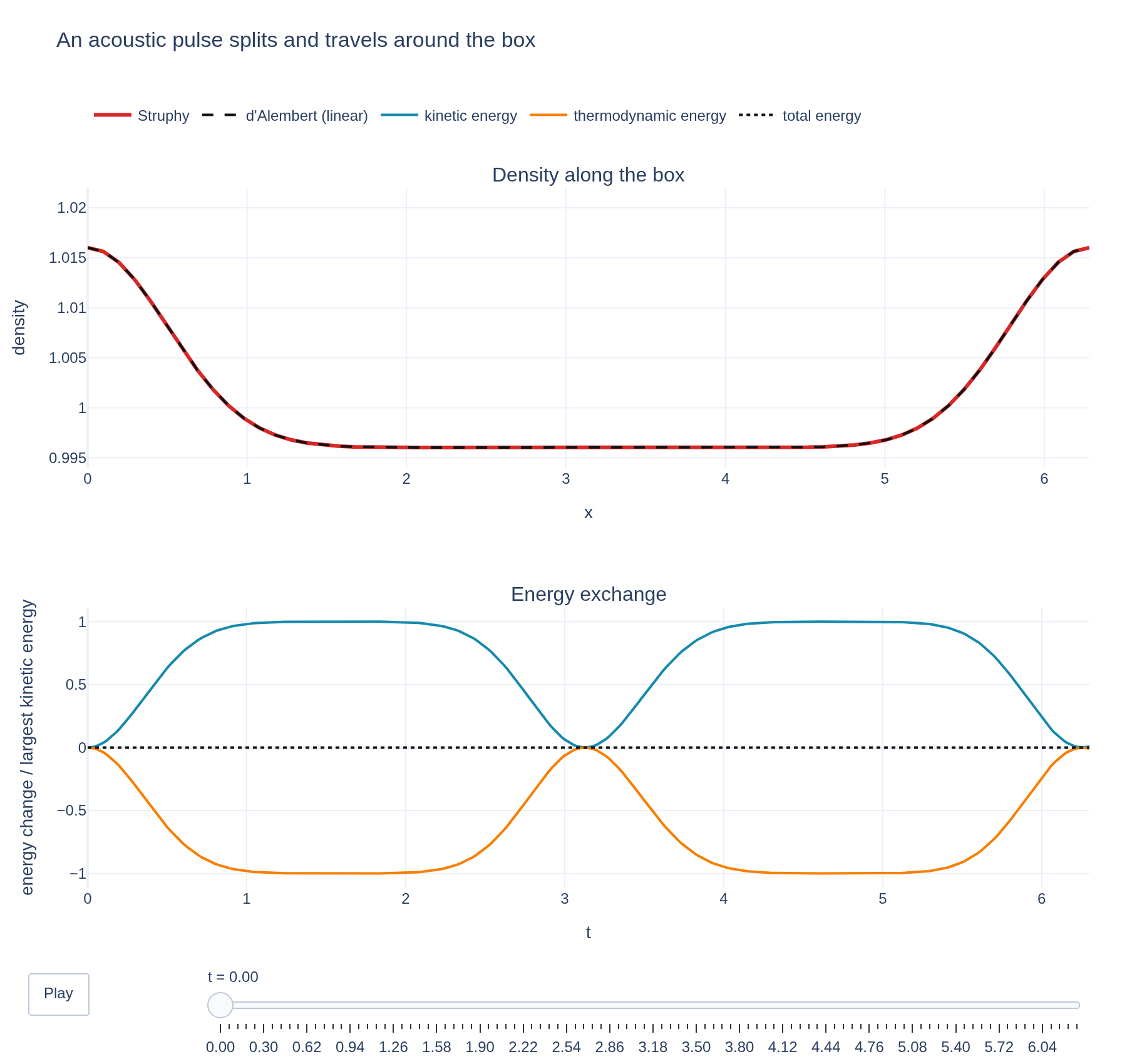
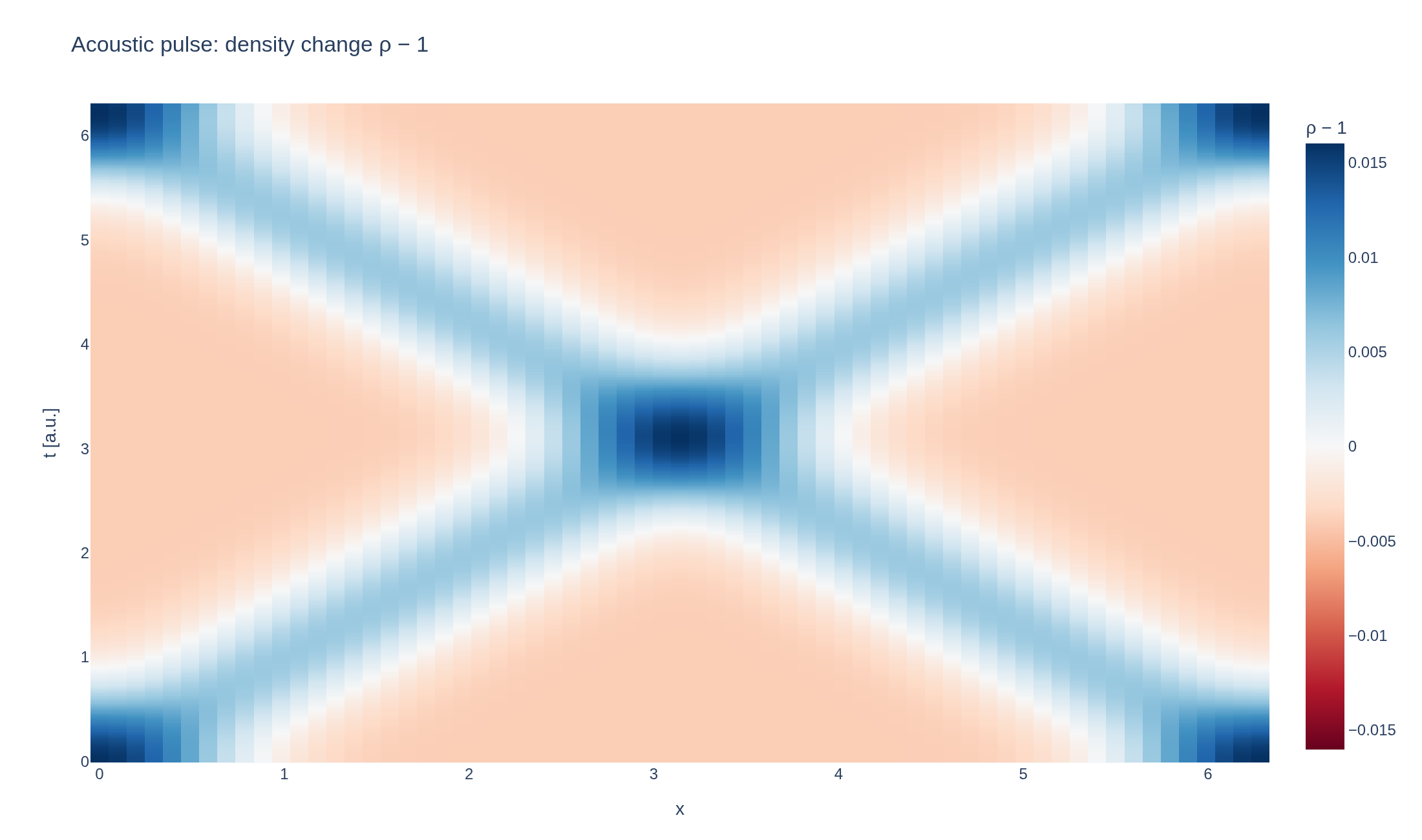
A Gaussian bump in the density of a compressible gas splits into two half-height pulses that travel in opposite directions at the speed of sound. Struphy's variational discretization follows them around the periodic box, conserving energy, and they agree with d'Alembert's solution.
Loading interactive figure…
Loading interactive figure…
Physical problem
A pulse that splits in two
PDEs solved by model:
Continuity:
Momentum:
Entropy:
where the internal energy per unit mass is .
Simulation geometry
Domain used in this run
The actual Cuboid geometry reconstructed from this run's metadata. Switch between the 3D view and physical-coordinate slices.
Domain
Cuboid
Mapping
Loading Cuboid…
Parameters
| Parameter | Value | Description |
|---|---|---|
| Loading parameters… | ||
Performance
Profiling
Struphy's built-in scope-profiler instruments every propagator, pusher and solver call — these are the real per-call timings from the run above.
Durations
Gantt (rank 0)
Region statistics
| Region | Count | Avg (s) | Min (s) | Max (s) | Total (s) |
|---|
Complete source
Simulation script
Requires Struphy with compiled kernels and Plotly. Run struphy compile once, then execute python acoustic-pulse.py.
"""An acoustic pulse in a compressible gas, with Struphy's VariationalCompressibleFluid model.

The gas has the pressure p = (gamma - 1) rho^gamma exp(s / rho), with gamma = 5/3 and an entropy chosen so that the
sound speed c = sqrt(gamma p / rho) is 1 at unit density. A Gaussian bump in the density (with the entropy per unit mass
left uniform), at rest, splits into two pulses of half the height that run in opposite directions at the speed of sound, cross
each other after the box has been traversed (the box is periodic), and reunite. For a small pulse the exact solution is
d'Alembert's, rho - 1 = (f(x - c t) + f(x + c t)) / 2. Struphy's variational discretization conserves the total energy: the pulse
starts as pure thermodynamic energy, which the running pulses share with kinetic energy.

Requires Struphy 3.3 with compiled kernels (`struphy compile`).
"""

import numpy as np
import plotly.graph_objects as go

from struphy import (
    DerhamOptions,
    EnvironmentOptions,
    FieldsBackground,
    Simulation,
    Time,
    domains,
    equils,
    grids,
    perturbations,
)
from struphy.linear_algebra.solver import NonlinearSolverParameters
from struphy.models import VariationalCompressibleFluid

length = 2 * np.pi
width = 0.5  # of the Gaussian pulse
amplitude = 0.02  # small, so that the pulse stays in the linear regime
modes = 10  # cosine modes that represent the Gaussian
sound_speed = 1.0
gamma = 5.0 / 3.0
# c^2 = gamma (gamma - 1) rho^(gamma - 1) exp(s / rho) equals 1 at unit density when exp(s / rho) = 1 / (gamma (gamma - 1)).
entropy_per_mass = -np.log(gamma * (gamma - 1.0))
time_opts = Time(dt=0.02, Tend=length / sound_speed, split_algo="Strang")  # one crossing of the periodic box
grid = grids.TensorProductGrid(num_elements=(64, 1, 1))
derham_opts = DerhamOptions(degree=(3, 1, 1))
domain = domains.Cuboid(l1=0.0, r1=length, l2=0.0, r2=1.0, l3=0.0, r3=1.0)

# The Gaussian, as a cosine series about x = 0 (the pulse wraps around the periodic box): f(x) = sum_n a_n cos(n k x).
harmonics = np.arange(1, modes + 1)
wavenumbers = 2 * np.pi * harmonics / length
coefficients = 2 * amplitude * width * np.sqrt(2 * np.pi) / length * np.exp(-0.5 * (wavenumbers * width) ** 2)


class CompatibleNonlinearSolverParameters(NonlinearSolverParameters):
    """Bridge Struphy code paths that use both attribute and mapping access."""

    def __getitem__(self, key):
        return getattr(self, key)


model = VariationalCompressibleFluid()
nonlinear_solver = CompatibleNonlinearSolverParameters(type="Newton")
model.propagators.variat_dens.options = model.propagators.variat_dens.Options(
    model="full", gamma=gamma, nonlin_solver=nonlinear_solver
)
model.propagators.variat_ent.options = model.propagators.variat_ent.Options(gamma=gamma, nonlin_solver=nonlinear_solver)
# Logical 3-forms include det(DF) = length, so a physical density 1 is the value `length`.
model.fluid.density.add_background(FieldsBackground(values=(length,)))
model.fluid.entropy.add_background(FieldsBackground(values=(entropy_per_mass * length,)))
model.fluid.velocity.add_background(FieldsBackground(values=(0.0, 0.0, 0.0)))
# The entropy per unit mass s / rho stays uniform, so the entropy follows the density: ds = (s / rho) d(rho).
for variable, factor in ((model.fluid.density, 1.0), (model.fluid.entropy, entropy_per_mass)):
    variable.add_perturbation(
        perturbations.ModesCos(
            ls=tuple(int(n) for n in harmonics), amps=tuple(float(factor * c) for c in coefficients), Lx=length,
            given_in_basis="physical",
        )
    )

sim = Simulation(
    model=model,
    name="Acoustic pulse",
    description=(
        "A Gaussian bump in the density of a compressible gas splits into two half-height pulses that travel in "
        "opposite directions at the speed of sound. Struphy's variational discretization follows them around the "
        "periodic box, conserving energy, and they agree with d'Alembert's solution."
    ),
    env=EnvironmentOptions(out_folders="struphy_gallery_runs", sim_folder="acoustic_pulse"),
    time_opts=time_opts,
    domain=domain,
    equil=equils.HomogenSlab(B0z=1.0, n0=1.0, beta=2.0),
    grid=grid,
    derham_opts=derham_opts,
)


def exact_density(x, t):
    """d'Alembert's solution of the linearized problem: the sum of the cosine modes, each oscillating at c k."""
    modes_x = np.cos(np.outer(np.atleast_1d(x), wavenumbers))
    return 1.0 + modes_x @ (coefficients * np.cos(sound_speed * wavenumbers * t))


if __name__ == "__main__":
    from plotly.subplots import make_subplots

    from _gallery import export_profiling, merge_metadata, save_extra_figure, save_figure, space_time_figure

    output = sim.run(profiling_activated=True)
    output.pproc(physical=True)

    rho = output.evaluate("fluid/density_xyz").isel(e2=0, e3=0)
    times = rho.t.values
    x = rho.e1.values * length
    density = rho.values
    exact = np.array([exact_density(x, t) for t in times])
    error = float(np.max(np.abs(density - exact)) / amplitude)
    print(f"Maximum error of the density, relative to the pulse height: {error:.3f}")

    kinetic = np.asarray(output.scalars["en_U"])
    thermo = np.asarray(output.scalars["en_thermo"])
    total = np.asarray(output.scalars["en_tot"])
    scalar_times = np.asarray(output.time)[: len(total)]
    energy_drift = float(np.max(np.abs(total / total[0] - 1.0)))
    print(f"Maximum relative drift of the total energy: {energy_drift:.2e}")
    energy_scale = float(kinetic.max())  # the largest kinetic energy the pulse reaches

    def profile_traces(index):
        return [
            go.Scatter(x=x, y=density[index], mode="lines", name="Struphy", line={"color": "#d62828", "width": 3}),
            go.Scatter(x=x, y=exact[index], mode="lines", name="d'Alembert (linear)",
                       line={"color": "#111", "width": 2, "dash": "dash"}),
        ]

    picks = np.unique(np.linspace(0, len(times) - 1, min(100, len(times)), dtype=int))
    figure = make_subplots(rows=2, cols=1, vertical_spacing=0.2,
                           subplot_titles=("Density along the box", "Energy exchange"))
    for trace in profile_traces(0):
        figure.add_trace(trace, row=1, col=1)
    figure.add_scatter(x=scalar_times, y=(kinetic - kinetic[0]) / energy_scale, mode="lines",
                       name="kinetic energy", line={"color": "#168aad", "width": 2}, row=2, col=1)
    figure.add_scatter(x=scalar_times, y=(thermo - thermo[0]) / energy_scale, mode="lines",
                       name="thermodynamic energy", line={"color": "#f77f00", "width": 2}, row=2, col=1)
    figure.add_scatter(x=scalar_times, y=(total - total[0]) / energy_scale, mode="lines",
                       name="total energy", line={"color": "#111", "width": 2, "dash": "dot"}, row=2, col=1)
    figure.frames = [go.Frame(name=f"{times[i]:.2f}", data=profile_traces(i), traces=[0, 1]) for i in picks]
    figure.update_layout(
        title="An acoustic pulse splits and travels around the box", template="plotly_white",
        margin={"l": 70, "r": 30, "t": 150, "b": 140}, title_y=0.97, legend={"orientation": "h", "y": 1.13},
        updatemenus=[{"type": "buttons", "showactive": False, "x": 0, "y": -0.12,
                      "buttons": [{"label": "Play", "method": "animate", "args": [None, {"frame": {"duration": 50, "redraw": False}, "transition": {"duration": 0}, "fromcurrent": True}]}]}],
        sliders=[{"active": 0, "x": 0.12, "len": 0.88, "y": -0.07, "currentvalue": {"prefix": "t = "},
                  "steps": [{"args": [[frame.name], {"frame": {"duration": 0, "redraw": False}, "transition": {"duration": 0}, "mode": "immediate"}], "label": frame.name, "method": "animate"} for frame in figure.frames]}],
    )
    figure.update_xaxes(title_text="x", range=[0, length], row=1, col=1)
    figure.update_yaxes(title_text="density", range=[1 - 0.3 * amplitude, 1 + 1.1 * amplitude], row=1, col=1)
    figure.update_xaxes(title_text="t", row=2, col=1)
    figure.update_yaxes(title_text="energy change / largest kinetic energy", row=2, col=1)
    save_figure(figure, "acoustic-pulse", width=900, height=850)

    density_change = rho.copy(data=density - 1.0)
    space_time = space_time_figure(
        density_change, space="e1", x_values=x, xaxis_title="x", title="Acoustic pulse: density change ρ − 1",
        colorbar_title="ρ − 1",
    )
    figures = [
        save_extra_figure(
            space_time, "acoustic-pulse", "space-time",
            alt="Space-time map of the density change of an acoustic pulse splitting into two",
            caption=(
                "The density change of the run above along x, over time. The pulse splits into two, and the two travelling "
                "pulses leave straight lines whose slope is the speed of sound, c = 1; because the box is periodic, they meet "
                "again on the opposite side at t = L / (2c)."
            ),
        ),
    ]

    merge_metadata(
        "acoustic-pulse",
        soundSpeed=sound_speed,
        maxRelativeError=error,
        maxEnergyDrift=energy_drift,
        figures=figures,
        **export_profiling(sim, "acoustic-pulse"),
    )
See the post-processing guide for more ways to inspect the result.