VlasovAmpereOneSpecies · Kinetic electrostatics
Langmuir wave dispersion
A density perturbation in a uniform Maxwellian plasma oscillates as a Langmuir wave and is Landau damped. Runs at four wavenumbers give the oscillation frequency and the damping rate against k, and are compared with the root of the kinetic dispersion relation and with the fluid Bohm–Gross estimate.
Loading interactive figure…
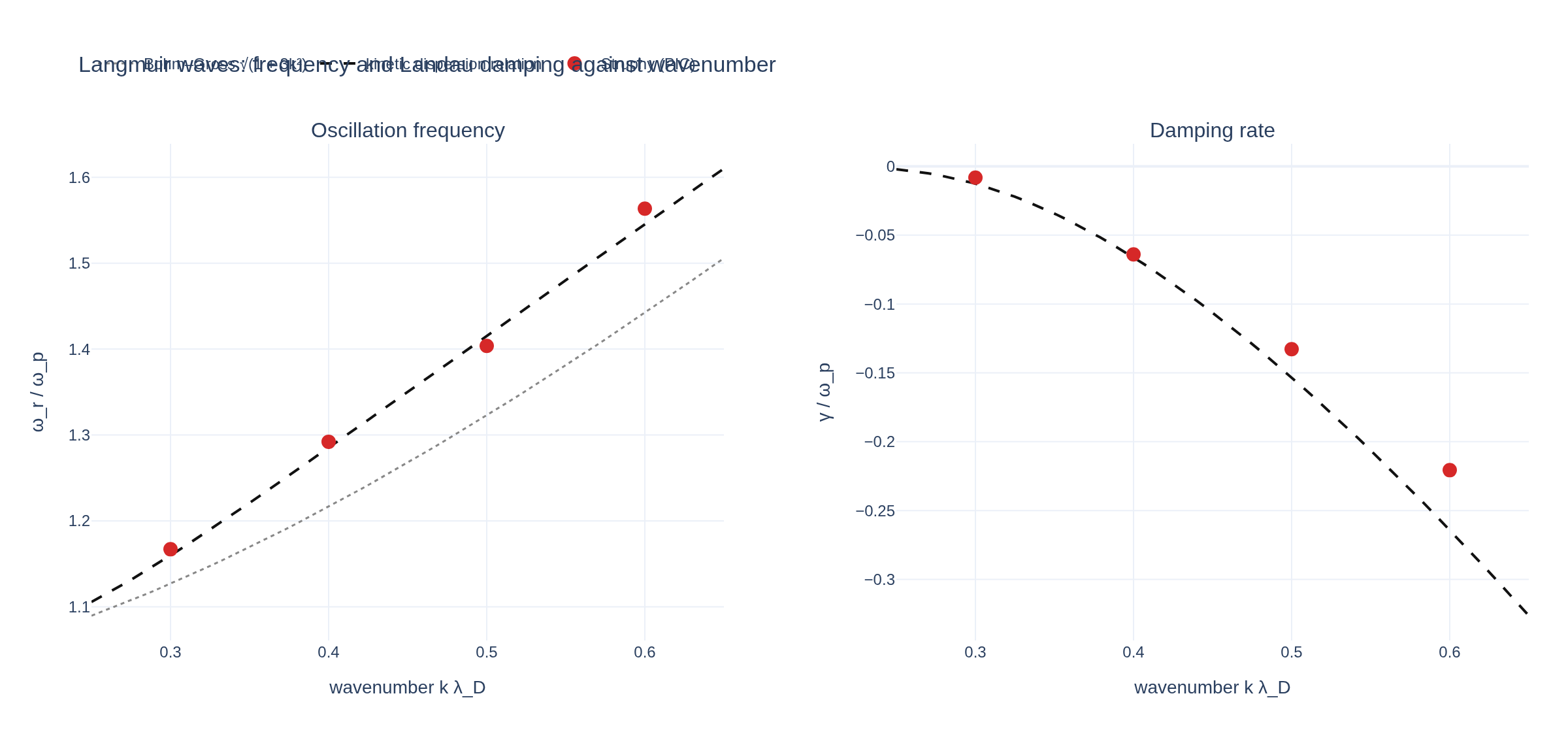
Loading interactive figure…
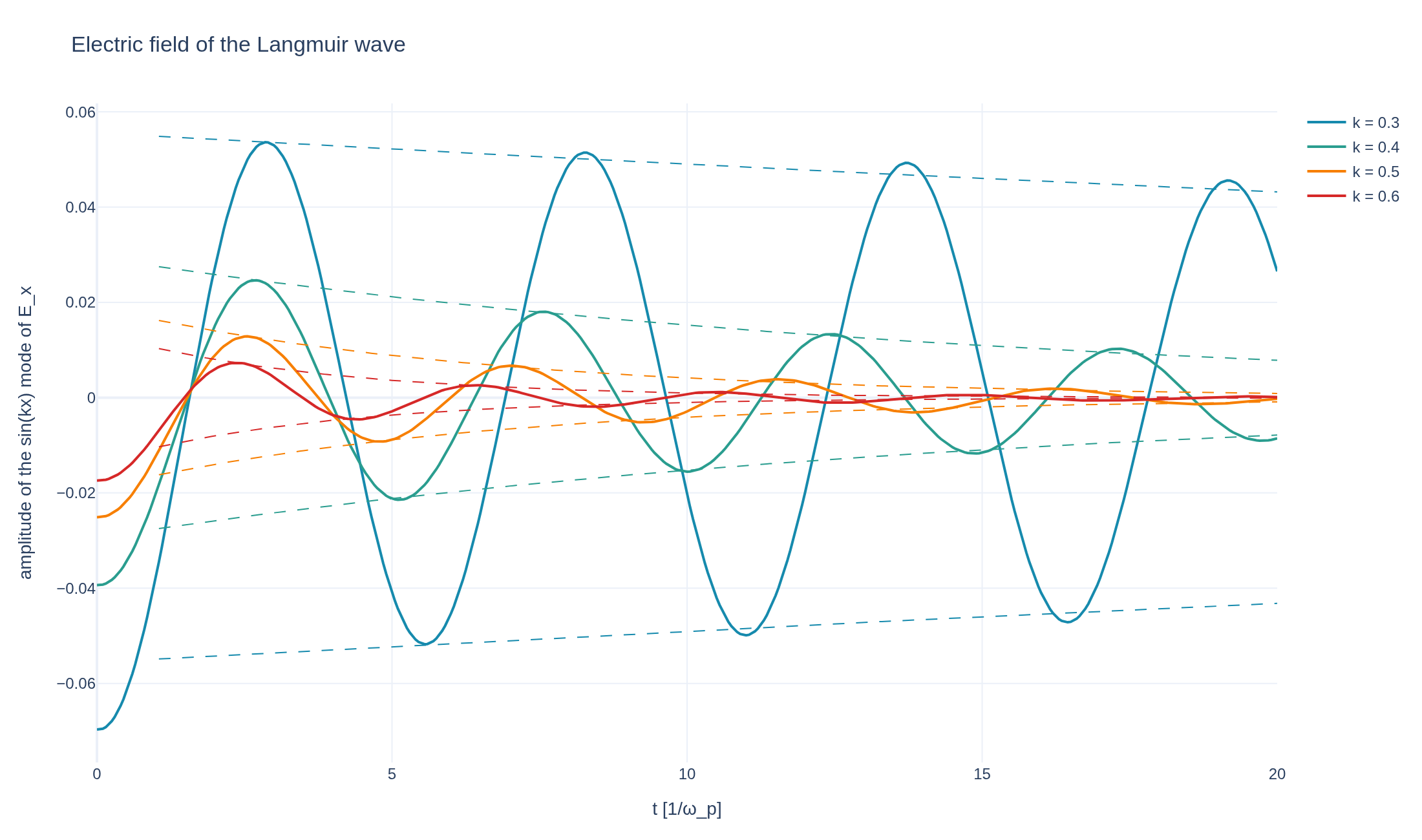
Physical problem
Frequency and damping of Langmuir waves
PDEs solved by model:
Vlasov equation:
Ampère's law:
Initial Poisson equation: At , solve weakly for the electric potential :
Simulation geometry
Domain used in this run
The actual Cuboid geometry reconstructed from this run's metadata. Switch between the 3D view and physical-coordinate slices.
Domain
Cuboid
Mapping
Loading Cuboid…
Parameters
| Parameter | Value | Description |
|---|---|---|
| Loading parameters… | ||
Performance
Profiling
Struphy's built-in scope-profiler instruments every propagator, pusher and solver call — these are the real per-call timings from the run above.
Durations
Gantt (rank 0)
Region statistics
| Region | Count | Avg (s) | Min (s) | Max (s) | Total (s) |
|---|
Complete source
Simulation script
Requires Struphy with compiled kernels and Plotly. Run struphy compile once, then execute python langmuir-wave-dispersion.py.
"""Langmuir waves and their Landau damping at several wavenumbers, with Struphy's VlasovAmpereOneSpecies model.

A small electrostatic density perturbation cos(k x) in a uniform Maxwellian plasma (thermal speed 1, plasma frequency 1) oscillates as a Langmuir wave, at a
frequency above the plasma frequency because of the thermal motion, while it is damped by Landau damping. The complex
frequency omega(k) = omega_r + i gamma is the root of the Vlasov dispersion relation

    1 + (1 + zeta Z(zeta)) / k^2 = 0,   zeta = omega / (sqrt(2) k),

with the plasma dispersion function Z. Four runs with wavenumbers between 0.3 and 0.6 (different box lengths) measure the oscillation
frequency and the damping rate of the electric field, and compare them with this root. The fluid estimate omega^2 = 1 + 3 k^2 (Bohm-Gross) is
shown for reference: it ignores the kinetic effects and misses the frequency by several per cent already at k = 0.5.

Requires Struphy 3.3 with compiled kernels (`struphy compile`).
"""

import numpy as np
import plotly.graph_objects as go
from scipy.optimize import fsolve
from scipy.special import wofz

from struphy import (
    BoundaryParameters,
    DerhamOptions,
    EnvironmentOptions,
    LoadingParameters,
    SavingParameters,
    Simulation,
    SortingParameters,
    Time,
    WeightsParameters,
    domains,
    grids,
    maxwellians,
    perturbations,
)
from struphy.models import VlasovAmpereOneSpecies

wavenumbers = (0.3, 0.4, 0.5, 0.6)  # the scan; the example itself is the k = 0.5 run
amplitude = 0.001
grid = grids.TensorProductGrid(num_elements=(32, 1, 1))
derham_opts = DerhamOptions(degree=(3, 1, 1))
time_opts = Time(dt=0.05, Tend=20.0, split_algo="LieTrotter")


def kinetic_frequency(k, guess=(1.4, -0.15)):
    """The complex Langmuir frequency, as (omega_r, gamma), from the root of the Vlasov dispersion relation."""

    def dispersion(values):
        zeta = (values[0] + 1j * values[1]) / (np.sqrt(2) * k)
        residual = 1 + (1 + zeta * 1j * np.sqrt(np.pi) * wofz(zeta)) / k**2
        return [residual.real, residual.imag]

    return fsolve(dispersion, guess, xtol=1e-12)


def make_simulation(k, folder, **extra):
    """Vlasov-Ampère in a periodic box of length 2 pi / k with one cosine mode in the density."""
    model = VlasovAmpereOneSpecies(alpha=1.0, epsilon=-1.0, with_B0=False)
    model.em_fields.e_field.save_data = True
    model.kinetic_ions.set_markers(
        loading_params=LoadingParameters(ppc=1000),
        weights_params=WeightsParameters(control_variate=True),
        boundary_params=BoundaryParameters(),
        sorting_params=SortingParameters(boxes_per_dim=(16, 1, 1), do_sort=True),
        saving_params=SavingParameters(),
        bufsize=2.0,
    )
    model.propagators.push_eta.options = model.propagators.push_eta.Options()
    model.propagators.coupling_va.options = model.propagators.coupling_va.Options()
    model.initial_poisson.options = model.initial_poisson.Options(stab_mat="M0")
    model.kinetic_ions.var.add_background(maxwellians.Maxwellian3D(n=(1.0, None)))
    mode = perturbations.ModesCos(amps=(amplitude,), ls=(1,))
    model.kinetic_ions.var.add_initial_condition(maxwellians.Maxwellian3D(n=(1.0, mode)))
    return Simulation(
        model=model,
        env=EnvironmentOptions(out_folders="struphy_gallery_runs", sim_folder=folder),
        time_opts=time_opts,
        domain=domains.Cuboid(r1=2 * np.pi / k),
        grid=grid,
        derham_opts=derham_opts,
        **extra,
    )


sim = make_simulation(
    0.5,
    "langmuir_wave_dispersion",
    name="Langmuir wave dispersion",
    description=(
        "A density perturbation in a uniform Maxwellian plasma oscillates as a Langmuir wave and is Landau damped. "
        "Runs at four wavenumbers give the oscillation frequency and the damping rate against k, and are compared with "
        "the root of the kinetic dispersion relation and with the fluid Bohm–Gross estimate."
    ),
)


def mode_amplitude(run):
    """Time and the amplitude of the sin(k x) mode of the electric field E_x, from a post-processed run."""
    e_x = run.evaluate("em_fields/e_field").isel(component=0, e2=0, e3=0)
    e1 = e_x.e1.values
    return e_x.t.values, 2.0 * np.mean(e_x.values[:, :-1] * np.sin(2 * np.pi * e1[:-1]), axis=1)


if __name__ == "__main__":
    from _gallery import export_profiling, is_root, merge_metadata, save_extra_figure, save_figure

    runs = {0.5: sim.run(profiling_activated=True)}
    for k in wavenumbers:
        if k != 0.5:
            runs[k] = make_simulation(k, f"langmuir_wave_dispersion_k{k}").run()
    for run in runs.values():
        run.pproc()

    exact, measured_frequency, measured_rate, amplitudes = {}, {}, {}, {}
    guess = (1.4, -0.15)
    for k in sorted(runs):
        exact[k] = kinetic_frequency(k, guess)
        guess = tuple(exact[k])
        times, values = mode_amplitude(runs[k])
        amplitudes[k] = values
        # The first time units hold a transient of phase-mixing modes that are not the Langmuir wave, so the fit starts at t = 1
        # and stops at t = 12. The measured values depend on this window at the level of a few per cent.
        window = (times > 1.0) & (times < 12.0)
        in_window = np.flatnonzero(window)
        crossings = in_window[:-1][np.diff(np.sign(values[in_window])) != 0]
        roots = times[crossings] - values[crossings] * (times[crossings + 1] - times[crossings]) / (
            values[crossings + 1] - values[crossings]
        )
        measured_frequency[k] = float(np.pi / np.mean(np.diff(roots)))
        magnitude = np.abs(values)
        peaks = np.where(window[1:-1] & (magnitude[1:-1] >= magnitude[:-2]) & (magnitude[1:-1] >= magnitude[2:]))[0] + 1
        measured_rate[k] = float(np.polyfit(times[peaks], np.log(magnitude[peaks]), 1)[0])
    if not (np.isfinite(list(measured_frequency.values())).all() and np.isfinite(list(measured_rate.values())).all()):
        raise RuntimeError("A frequency or a damping rate could not be measured")
    if is_root():
        for k in sorted(runs):
            print(f"k = {k}: omega_r = {measured_frequency[k]:.4f} (kinetic {exact[k][0]:.4f}), "
                  f"gamma = {measured_rate[k]:.4f} (kinetic {exact[k][1]:.4f})")

    from plotly.subplots import make_subplots

    k_line = np.linspace(0.25, 0.65, 60)
    lines, guess = [], (1.15, -0.01)
    for kk in k_line:
        guess = tuple(kinetic_frequency(kk, guess))
        lines.append(guess)
    lines = np.array(lines)
    ks = sorted(runs)
    figure = make_subplots(rows=1, cols=2, horizontal_spacing=0.12,
                           subplot_titles=("Oscillation frequency", "Damping rate"))
    figure.add_scatter(x=k_line, y=np.sqrt(1 + 3 * k_line**2), mode="lines", name="Bohm–Gross √(1 + 3k²)",
                       line={"color": "#888", "width": 1.5, "dash": "dot"}, row=1, col=1)
    figure.add_scatter(x=k_line, y=lines[:, 0], mode="lines", name="kinetic dispersion relation",
                       line={"color": "#111", "width": 2, "dash": "dash"}, row=1, col=1)
    figure.add_scatter(x=ks, y=[measured_frequency[k] for k in ks], mode="markers", name="Struphy (PIC)",
                       marker={"color": "#d62828", "size": 11}, row=1, col=1)
    figure.add_scatter(x=k_line, y=lines[:, 1], mode="lines", showlegend=False,
                       line={"color": "#111", "width": 2, "dash": "dash"}, row=1, col=2)
    figure.add_scatter(x=ks, y=[measured_rate[k] for k in ks], mode="markers", showlegend=False,
                       marker={"color": "#d62828", "size": 11}, row=1, col=2)
    figure.update_layout(
        title="Langmuir waves: frequency and Landau damping against wavenumber", template="plotly_white",
        margin={"l": 70, "r": 30, "t": 110, "b": 70}, legend={"orientation": "h", "y": 1.2},
    )
    figure.update_xaxes(title_text="wavenumber k λ_D")
    figure.update_yaxes(title_text="ω_r / ω_p", row=1, col=1)
    figure.update_yaxes(title_text="γ / ω_p", row=1, col=2)
    save_figure(figure, "langmuir-wave-dispersion", width=1200, height=560)

    colors = {0.3: "#168aad", 0.4: "#2a9d8f", 0.5: "#f77f00", 0.6: "#d62828"}
    signals = go.Figure()
    for k in ks:
        times, _ = mode_amplitude(runs[k])
        # The exact envelope exp(gamma t), scaled to the first peak of the wave (after the initial transient).
        after = times > 1.0
        first_peak = np.argmax(np.abs(amplitudes[k][after][:40]))
        t_peak = times[after][first_peak]
        scale = abs(amplitudes[k][after][first_peak]) * np.exp(-exact[k][1] * t_peak)
        signals.add_scatter(x=times, y=amplitudes[k], mode="lines", name=f"k = {k}", line={"color": colors[k], "width": 2})
        for sign in (1, -1):
            signals.add_scatter(x=times[after], y=sign * scale * np.exp(exact[k][1] * times[after]), mode="lines",
                                showlegend=False, line={"color": colors[k], "width": 1, "dash": "dash"})
    signals.update_layout(
        title="Electric field of the Langmuir wave", template="plotly_white", autosize=True,
        xaxis_title="t [1/ω_p]", yaxis_title="amplitude of the sin(kx) mode of E_x",
        margin={"l": 75, "r": 30, "t": 80, "b": 60},
    )
    figures = [
        save_extra_figure(
            signals, "langmuir-wave-dispersion", "signals",
            alt="Electric field of Langmuir waves at four wavenumbers, damped inside their Landau envelopes",
            caption=(
                "The amplitude of the electric field mode in the four runs, with the Landau envelope exp(γt) (γ from the kinetic dispersion "
                "relation, scaled to the first peak) as dashed lines. The wave oscillates faster and dies out sooner as k grows. The first "
                "time units hold a transient of phase-mixing modes that are not the Langmuir wave, so the frequencies and rates above are "
                "read from t = 1 to t = 12."
            ),
        ),
    ]

    merge_metadata(
        "langmuir-wave-dispersion",
        waves={str(k): {"measuredFrequency": measured_frequency[k], "kineticFrequency": float(exact[k][0]),
                        "measuredRate": measured_rate[k], "kineticRate": float(exact[k][1])} for k in ks},
        figures=figures,
        **export_profiling(sim, "langmuir-wave-dispersion"),
    )
See the post-processing guide for more ways to inspect the result.