Poisson · Electrostatics
Poisson convergence on a distorted mesh
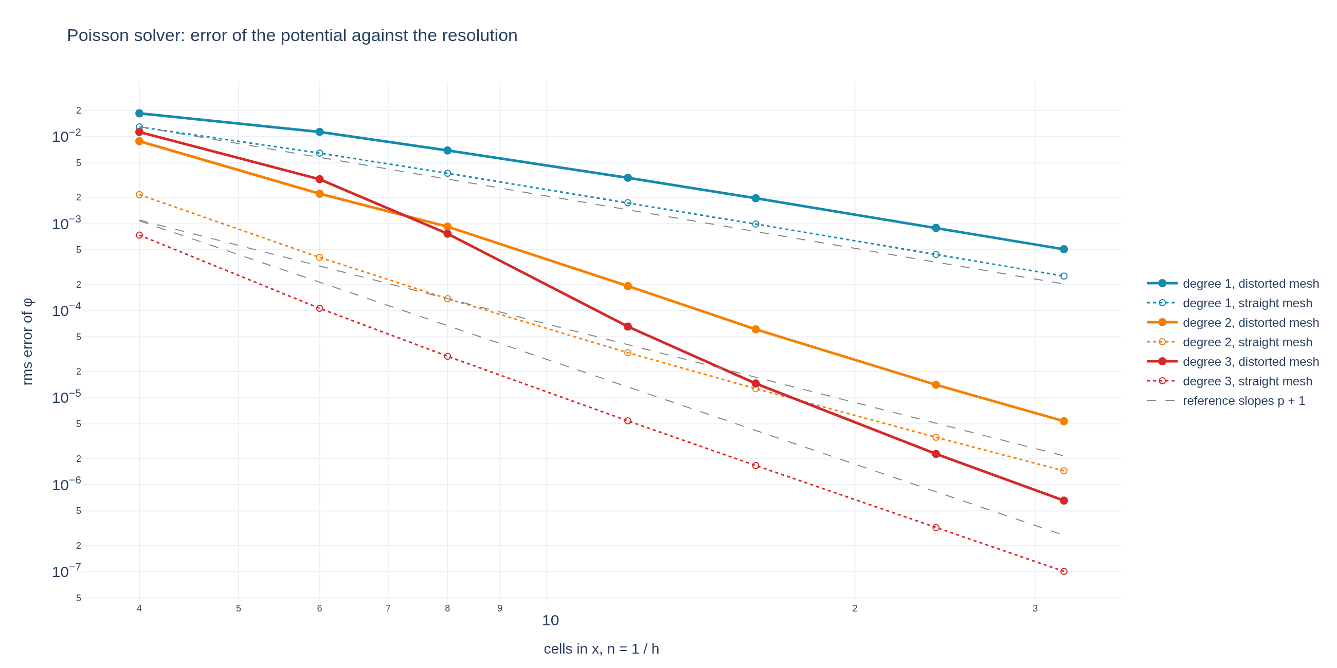
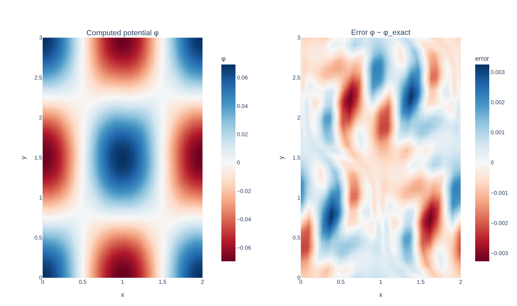
A cosine source on a periodic box, solved with splines of degree 1 to 3 on a mesh that the Colella mapping has bent. The error of the potential against the exact solution falls with the mesh width h at least as fast as h^(p+1) for a spline degree p, on the curved mesh as well as on the straight one.
Loading interactive figure…
Loading interactive figure…
Physical problem
Error against resolution on a bent mesh
PDEs solved by model:
Find such that
where are real-valued functions, is parametrized by time , and is a positive matrix. Boundary terms from integration by parts are assumed to vanish.
Simulation geometry
Domain used in this run
The actual Colella geometry reconstructed from this run's metadata. Switch between the 3D view and physical-coordinate slices.
Domain
Colella
Mapping
Loading Colella…
Parameters
| Parameter | Value | Description |
|---|---|---|
| Loading parameters… | ||
Performance
Profiling
Struphy's built-in scope-profiler instruments every propagator, pusher and solver call — these are the real per-call timings from the run above.
Durations
Gantt (rank 0)
Region statistics
| Region | Count | Avg (s) | Min (s) | Max (s) | Total (s) |
|---|
Complete source
Simulation script
Requires Struphy with compiled kernels and Plotly. Run struphy compile once, then execute python poisson-convergence.py.
"""Convergence of Struphy's Poisson solver on a distorted mesh.

The equation -Laplace(phi) = rho with the source rho = cos(kx x) cos(ky y) on the periodic box [0, 2] x [0, 3] has the exact solution
phi = rho / (kx^2 + ky^2). Struphy solves it with continuous finite elements (splines) of degree p on a mesh of n x 1.5 n cells, and the
Colella mapping bends the mesh lines inside the box (leaving the box itself where it is) by an amount alpha. The error of the potential
falls at least as fast as h^(p+1) in the root-mean-square norm when the mesh is refined, at every degree, on the straight mesh (alpha = 0) and on
the curved one. The slopes are measured from the runs and compared with p + 1: on the straight mesh they are close to it, and on the curved mesh,
whose coarse meshes are not yet in the asymptotic range, they are steeper.

Requires Struphy 3.3 with compiled kernels (`struphy compile`).
"""

import numpy as np
import plotly.graph_objects as go

from struphy import DerhamOptions, EnvironmentOptions, Simulation, Time, domains, grids
from struphy.initial.base import GenericPerturbation
from struphy.linear_algebra.solver import SolverParameters
from struphy.models import Poisson

lx, ly = 2.0, 3.0
kx, ky = 2 * np.pi / lx, 2 * np.pi / ly
distortion = 0.1
degrees = (1, 2, 3)
resolutions = (4, 6, 8, 12, 16, 24, 32)  # cells in x; there are 1.5 times as many in y
time_opts = Time(dt=0.1, Tend=0.1)  # the potential is found before the first time step, and again at each step


def source(x, y, z):
    return np.cos(kx * x) * np.cos(ky * y)


def exact_potential(x, y):
    return source(x, y, 0.0) / (kx**2 + ky**2)


def make_simulation(degree, cells, alpha, folder, **extra):
    """The Poisson model on the Colella mesh with the distortion alpha, degree `degree` and `cells` x 1.5 `cells` elements."""
    model = Poisson()
    # A tight tolerance, so that the error of the linear solver stays below the discretization error at every resolution.
    model.propagators.poisson.options = model.propagators.poisson.Options(
        solver_params=SolverParameters(tol=1e-14, maxiter=5000)
    )
    model.em_fields.source.add_perturbation(GenericPerturbation(source, given_in_basis="physical"))
    return Simulation(
        model=model,
        env=EnvironmentOptions(out_folders="struphy_gallery_runs", sim_folder=folder),
        time_opts=time_opts,
        domain=domains.Colella(Lx=lx, Ly=ly, alpha=alpha, Lz=1.0),
        grid=grids.TensorProductGrid(num_elements=(cells, int(1.5 * cells), 1)),
        derham_opts=DerhamOptions(degree=(degree, degree, 1)),
        **extra,
    )


sim = make_simulation(
    2, 8, distortion, "poisson_convergence",
    name="Poisson convergence on a distorted mesh",
    description=(
        "A cosine source on a periodic box, solved with splines of degree 1 to 3 on a mesh that the Colella mapping has "
        "bent. The error of the potential against the exact solution falls with the mesh width h at least as fast as "
        "h^(p+1) for a spline degree p, on the curved mesh as well as on the straight one."
    ),
)


def potential_error(run):
    """Points and the difference between the computed and the exact potential at the last time, from a post-processed run."""
    phi = run.evaluate("em_fields/phi").isel(t=-1, e3=0)
    return phi.X.values, phi.Y.values, phi.values, phi.values - exact_potential(phi.X.values, phi.Y.values)


if __name__ == "__main__":
    from plotly.subplots import make_subplots
    from scipy.interpolate import griddata

    from _gallery import export_profiling, is_root, merge_metadata, save_extra_figure, save_figure

    sim.run(profiling_activated=True)

    errors = {}  # (alpha, degree) -> rms errors against the resolution
    for alpha in (distortion, 0.0):
        for degree in degrees:
            values = []
            for cells in resolutions:
                run = make_simulation(degree, cells, alpha, f"poisson_convergence_p{degree}_n{cells}_a{alpha}").run()
                run.pproc(physical=True, celldivide=3)  # three sample points per cell, to measure the error inside the cells
                _, _, _, difference = potential_error(run)
                values.append(float(np.sqrt(np.mean(difference**2))))
            errors[(alpha, degree)] = np.array(values)
    if not all(np.isfinite(v).all() for v in errors.values()):
        raise RuntimeError("Non-finite errors")

    n = np.array(resolutions, dtype=float)  # the mesh width is h = 1 / n
    h = 1.0 / n
    # The slope of the last four resolutions, before the error reaches the level of the solver.
    slopes = {key: float(np.polyfit(np.log(h[-4:]), np.log(v[-4:]), 1)[0]) for key, v in errors.items()}
    if is_root():
        for (alpha, degree), slope in slopes.items():
            print(f"alpha = {alpha}, degree {degree}: slope {slope:.2f} (expected {degree + 1}), error at n = {resolutions[-1]}: "
                  f"{errors[(alpha, degree)][-1]:.2e}")

    colors = {1: "#168aad", 2: "#f77f00", 3: "#d62828"}
    figure = go.Figure()
    for degree in degrees:
        figure.add_scatter(x=n, y=errors[(distortion, degree)], mode="lines+markers", name=f"degree {degree}, distorted mesh",
                           line={"color": colors[degree], "width": 2.5}, marker={"size": 8})
        figure.add_scatter(x=n, y=errors[(0.0, degree)], mode="lines+markers", name=f"degree {degree}, straight mesh",
                           line={"color": colors[degree], "width": 1.5, "dash": "dot"},
                           marker={"size": 6, "symbol": "circle-open"})
    for degree in degrees:
        # A reference line of slope -(p + 1), through a point below the last one of the distorted-mesh curve.
        anchor = errors[(distortion, degree)][-1] * 0.4
        figure.add_scatter(x=[n[0], n[-1]], y=[anchor * (n[-1] / n[0]) ** (degree + 1), anchor], mode="lines",
                           name=f"slope {degree + 1}", line={"color": "#888", "width": 1, "dash": "dash"},
                           showlegend=(degree == 1))
        figure.data[-1].name = "reference slopes p + 1"
    figure.update_layout(
        title="Poisson solver: error of the potential against the resolution", template="plotly_white", autosize=True,
        xaxis_title="cells in x, n = 1 / h", yaxis_title="rms error of φ", xaxis_type="log", yaxis_type="log",
        legend={"x": 1.02, "y": 0.5}, margin={"l": 80, "r": 30, "t": 80, "b": 65},
    )
    save_figure(figure, "poisson-convergence", width=1300, height=650)

    # The solution and its error on the distorted mesh, at degree 2 and 8 x 12 cells.
    run = make_simulation(2, 8, distortion, "poisson_convergence_map").run()
    run.pproc(physical=True, celldivide=4)
    mesh_x, mesh_y, potential, difference = potential_error(run)
    x_plot, y_plot = np.linspace(0, lx, 100), np.linspace(0, ly, 150)
    xx, yy = np.meshgrid(x_plot, y_plot)
    points = np.column_stack([mesh_x.ravel(), mesh_y.ravel()])

    def resample(values):
        return griddata(points, values.ravel(), (xx, yy), method="linear")

    maps = make_subplots(rows=1, cols=2, horizontal_spacing=0.18, subplot_titles=("Computed potential φ", "Error φ − φ_exact"))
    maps.add_trace(go.Heatmap(z=resample(potential), x=x_plot, y=y_plot, colorscale="RdBu", zmid=0.0,
                              colorbar={"title": "φ", "x": 0.42, "len": 0.9}), row=1, col=1)
    limit = float(np.abs(difference).max())
    maps.add_trace(go.Heatmap(z=resample(difference), x=x_plot, y=y_plot, colorscale="RdBu", zmid=0.0, zmin=-limit, zmax=limit,
                              colorbar={"title": "error", "x": 1.0, "len": 0.9, "exponentformat": "e"}), row=1, col=2)
    for column in (1, 2):
        maps.update_xaxes(title_text="x", range=[0, lx], constrain="domain", row=1, col=column)
        maps.update_yaxes(title_text="y", range=[0, ly], scaleanchor=f"x{column}" if column > 1 else "x", row=1, col=column)
    maps.update_layout(template="plotly_white", autosize=True, margin={"l": 70, "r": 30, "t": 80, "b": 60})
    figures = [
        save_extra_figure(
            maps, "poisson-convergence", "maps",
            alt="Computed potential and its error on a distorted mesh of 8 by 12 cells with splines of degree 2",
            caption=(
                "The potential (left) and its error against the exact solution (right) for splines of degree 2 on the distorted mesh of "
                f"8 × 12 cells. The largest error is {limit:.1e}, {100 * limit / np.abs(potential).max():.2f} % of the peak of the potential, "
                "and it follows the pattern of the mesh."
            ),
        ),
    ]

    merge_metadata(
        "poisson-convergence",
        distortion=distortion,
        convergenceSlopes={f"degree {degree}": {"distorted": slopes[(distortion, degree)], "straight": slopes[(0.0, degree)],
                                                "expected": degree + 1} for degree in degrees},
        figures=figures,
        **export_profiling(sim, "poisson-convergence"),
    )
See the post-processing guide for more ways to inspect the result.