ViscoResistiveLinearMHD · Dissipative MHD
Viscous and resistive linear Alfvén wave
A standing Alfvén wave loses energy through both viscosity and resistivity in ViscoResistiveLinearMHD. Equal diffusivities give a simple exponential envelope for the oscillating velocity and magnetic field. Initially with on . Both diffusivities are ; the wave energy decays as .
Loading interactive figure…
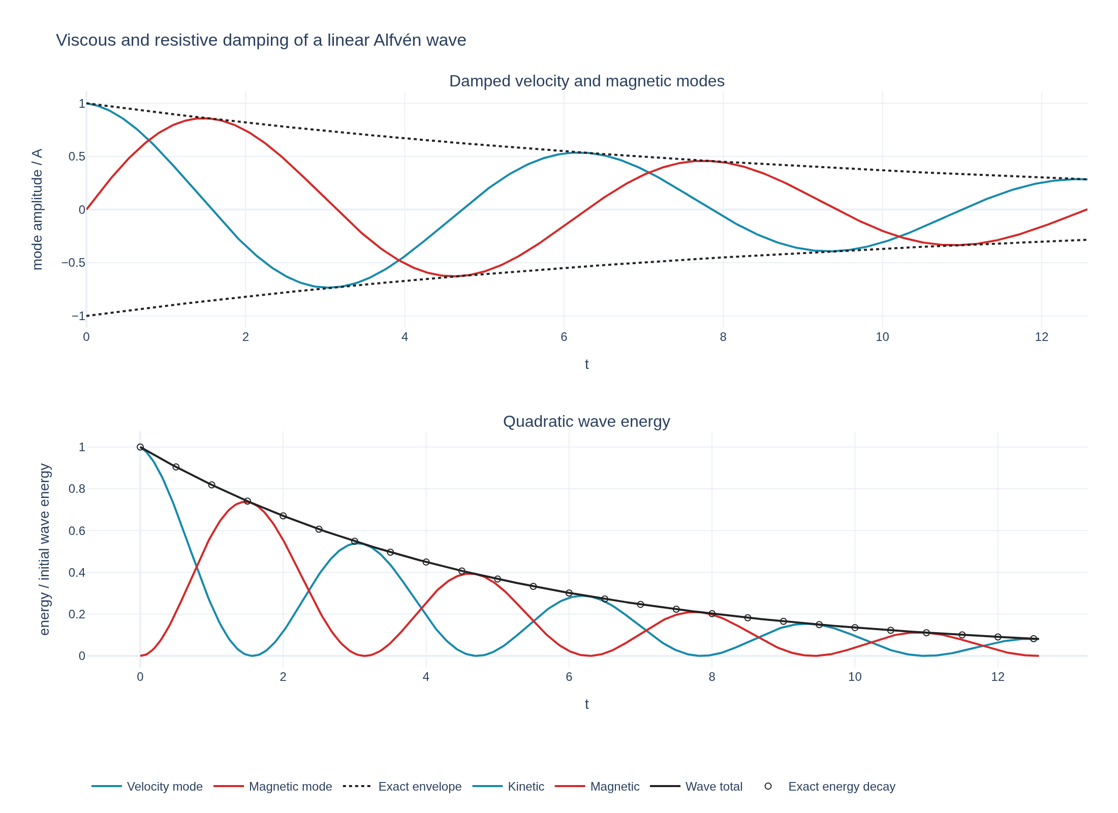
Loading interactive figure…
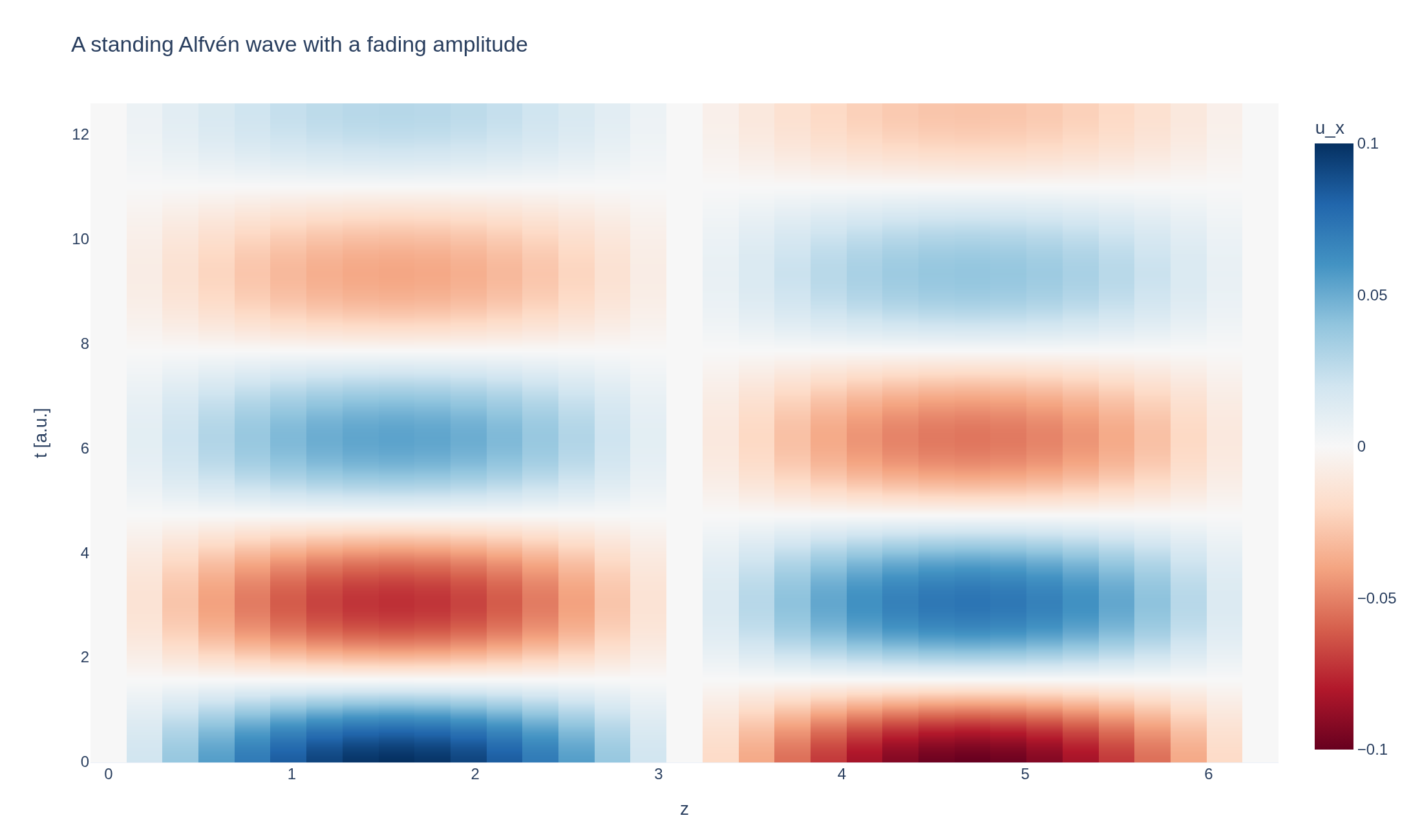
Physical problem
A standing wave with viscosity and resistivity
PDEs solved by model:
Continuity:
Momentum:
Pressure:
Induction:
Here and are artificial viscosity and resistivity coefficients.
Simulation geometry
Domain used in this run
The actual Cuboid geometry reconstructed from this run's metadata. Switch between the 3D view and physical-coordinate slices.
Domain
Cuboid
Mapping
Loading Cuboid…
Parameters
| Parameter | Value | Description |
|---|---|---|
| Loading parameters… | ||
Performance
Profiling
Struphy's built-in scope-profiler instruments every propagator, pusher and solver call — these are the real per-call timings from the run above.
Durations
Gantt (rank 0)
Region statistics
| Region | Count | Avg (s) | Min (s) | Max (s) | Total (s) |
|---|
Complete source
Simulation script
Requires Struphy with compiled kernels and Plotly. Run struphy compile once, then execute python linear-dissipative-alfven-wave.py.
"""A damped standing wave in ViscoResistiveLinearMHD.

Equal kinematic viscosity and magnetic diffusivity give the exact solution
u_x = A exp(-nu*k**2*t) sin(k*z) cos(k*t),
b_x = A exp(-nu*k**2*t) cos(k*z) sin(k*t), for B0 = rho0 = 1.
The linear model dissipates the quadratic wave energy; heating is second order
and is not part of this linear perturbation system.

Requires the pinned Struphy with compiled kernels (`struphy compile`).
"""

import numpy as np

from struphy import (
    DerhamOptions, EnvironmentOptions, Simulation, Time,
    domains, equils, grids, perturbations,
)
from struphy.models import ViscoResistiveLinearMHD

stem = "linear-dissipative-alfven-wave"
length, amplitude, diffusivity = 2.0 * np.pi, 0.1, 0.1
model = ViscoResistiveLinearMHD()
model.propagators.variat_dens.options = model.propagators.variat_dens.Options(model="linear")
model.propagators.variat_pb.options = model.propagators.variat_pb.Options(model="linear")
model.propagators.variat_viscous.options = model.propagators.variat_viscous.Options(model="linear_p", mu=diffusivity)
model.propagators.variat_resist.options = model.propagators.variat_resist.Options(model="linear_p", eta=diffusivity)
model.mhd.velocity.add_perturbation(
    perturbations.ModesSin(ns=(1,), amps=(amplitude,), comp=0, Lz=length, given_in_basis="physical"),
)
model.mhd.velocity.save_data = True
model.em_fields.b_field.save_data = True
domain = domains.Cuboid(r3=length)
grid = grids.TensorProductGrid(num_elements=(1, 1, 32))
derham_opts = DerhamOptions(degree=(1, 1, 3))
time_opts = Time(dt=0.025, Tend=2.0 * length, split_algo="Strang")
sim = Simulation(
    model=model,
    name="Viscous and resistive linear Alfvén wave",
    description=(
        "A standing Alfvén wave loses energy through both viscosity and resistivity in "
        "ViscoResistiveLinearMHD. Equal diffusivities give a simple exponential envelope "
        "for the oscillating velocity and magnetic field."
        r" Initially $$u_x(z,0)=0.1\sin z,\qquad\delta\mathbf{B}(z,0)=0,$$"
        r" with :math:`\rho_0=B_0=1` on :math:`0\leq z<2\pi`."
        r" Both diffusivities are :math:`\nu=\eta=0.1`; the wave energy decays as :math:`e^{-0.2t}`."
    ),
    env=EnvironmentOptions(out_folders="struphy_gallery_runs", sim_folder="linear_dissipative_alfven_wave"),
    time_opts=time_opts, domain=domain, grid=grid, derham_opts=derham_opts,
    equil=equils.HomogenSlab(B0z=1.0, n0=1.0, beta=0.1),
)


if __name__ == "__main__":
    from plotly.subplots import make_subplots

    from _gallery import export_profiling, merge_metadata, save_extra_figure, save_figure, space_time_figure

    output = sim.run(profiling_activated=True)
    output.pproc(physical=True)
    velocity = output.evaluate("mhd/velocity_xyz").isel(component=0, e1=0, e2=0)
    magnetic = output.evaluate("em_fields/b_field_xyz").isel(component=0, e1=0, e2=0)
    kinetic = output.evaluate("en_U")
    magnetic_energy = output.evaluate("en_mag_1")
    times, z = velocity.t.values, velocity.e3.values * length
    if not all(np.isfinite(a.values).all() for a in (velocity, magnetic, kinetic, magnetic_energy)):
        raise RuntimeError("The linear MHD run produced non-finite diagnostics")
    if abs(times[-1] - time_opts.Tend) > time_opts.dt:
        raise RuntimeError("The linear MHD run did not reach the requested end time")
    exact_u = amplitude * np.exp(-diffusivity * times[:, None]) * np.cos(times[:, None]) * np.sin(z[None, :])
    exact_b = amplitude * np.exp(-diffusivity * times[:, None]) * np.sin(times[:, None]) * np.cos(z[None, :])
    error = float(max(np.max(np.abs(velocity.values - exact_u)), np.max(np.abs(magnetic.values - exact_b))) / amplitude)
    energy_time = kinetic.t.values
    wave_energy = kinetic.values + magnetic_energy.values
    exact_energy = np.exp(-2.0 * diffusivity * energy_time)
    energy_error = float(np.max(np.abs(wave_energy / wave_energy[0] - exact_energy)))
    if max(error, energy_error) > 0.03:
        raise RuntimeError(f"The dissipative Alfvén wave differs from its exact solution: field={error:.3g}, energy={energy_error:.3g}")
    # The periodic evaluation grid repeats its endpoint; exclude it from mode projections.
    u_mode = 2 * np.mean(velocity.values[:, :-1] * np.sin(z[:-1]), axis=1) / amplitude
    b_mode = 2 * np.mean(magnetic.values[:, :-1] * np.cos(z[:-1]), axis=1) / amplitude
    figure = make_subplots(rows=2, cols=1, vertical_spacing=0.18,
                           subplot_titles=("Damped velocity and magnetic modes", "Quadratic wave energy"))
    for values, label, color in ((u_mode, "Velocity mode", "#168aad"), (b_mode, "Magnetic mode", "#d62828")):
        figure.add_scatter(x=times, y=values, name=label, line={"color": color}, row=1, col=1)
    for sign in (-1, 1):
        figure.add_scatter(x=times, y=sign * np.exp(-diffusivity * times), name="Exact envelope",
                           showlegend=sign == 1, line={"color": "#222", "dash": "dot"}, row=1, col=1)
    for values, label, color in ((kinetic.values, "Kinetic", "#168aad"),
                                 (magnetic_energy.values, "Magnetic", "#d62828"), (wave_energy, "Wave total", "#222")):
        figure.add_scatter(x=energy_time, y=values / wave_energy[0], name=label, line={"color": color}, row=2, col=1)
    figure.add_scatter(x=energy_time[::20], y=exact_energy[::20], mode="markers", name="Exact energy decay",
                       marker={"color": "#222", "symbol": "circle-open"}, row=2, col=1)
    figure.update_xaxes(title_text="t")
    figure.update_yaxes(title_text="mode amplitude / A", row=1, col=1)
    figure.update_yaxes(title_text="energy / initial wave energy", row=2, col=1)
    figure.update_layout(title="Viscous and resistive damping of a linear Alfvén wave", template="plotly_white",
                         legend={"orientation": "h", "y": -0.18}, margin={"l": 85, "r": 30, "t": 90, "b": 140})
    save_figure(figure, stem, height=800)
    space_time = space_time_figure(velocity, space="e3", x_values=z, xaxis_title="z",
                                   title="A standing Alfvén wave with a fading amplitude", colorbar_title="u_x")
    figures = [save_extra_figure(space_time, stem, "space-time", alt="Standing Alfvén wave fading under viscosity and resistivity",
                                caption="The nodes remain fixed while viscosity and resistivity damp the wave.")]
    merge_metadata(stem, maxRelativeFieldError=error, maxRelativeEnergyError=energy_error,
                   figures=figures, **export_profiling(sim, stem))
See the post-processing guide for more ways to inspect the result.