LinearMHDVlasovCC · Hybrid kinetic-MHD
Alfvén wave with kinetic-ion current coupling
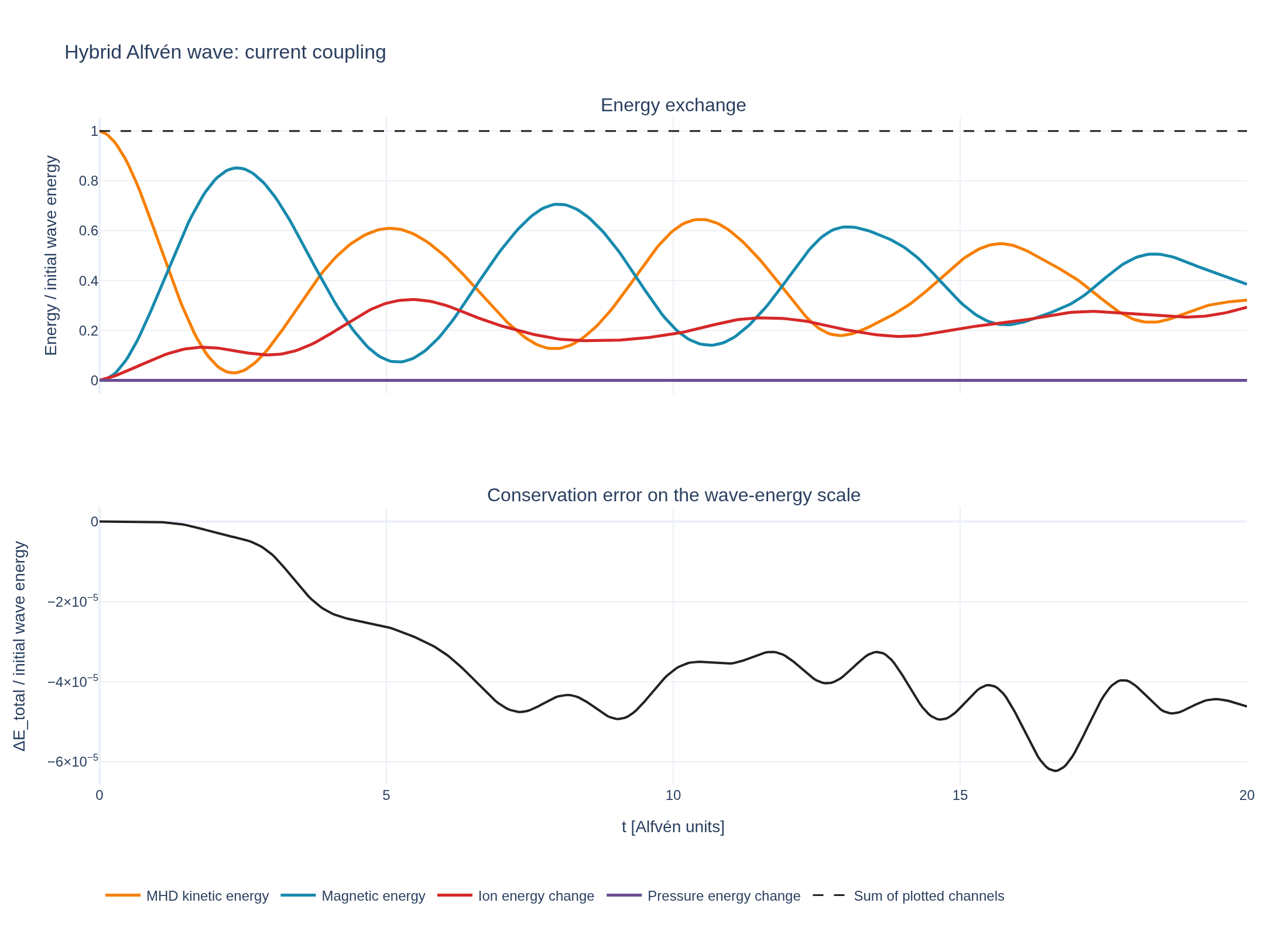
A shear-Alfvén wave exchanges energy with a dilute population of kinetic ions. The LinearMHDVlasovCC hybrid model evolves the bulk plasma as a fluid and the energetic ions as particles, coupled through their current. Follow the wave and compare energy transfer with the total-energy conservation error. The fluid starts with in , . The energetic-ion Maxwellian has , and isotropic thermal speed .
Loading interactive figure…
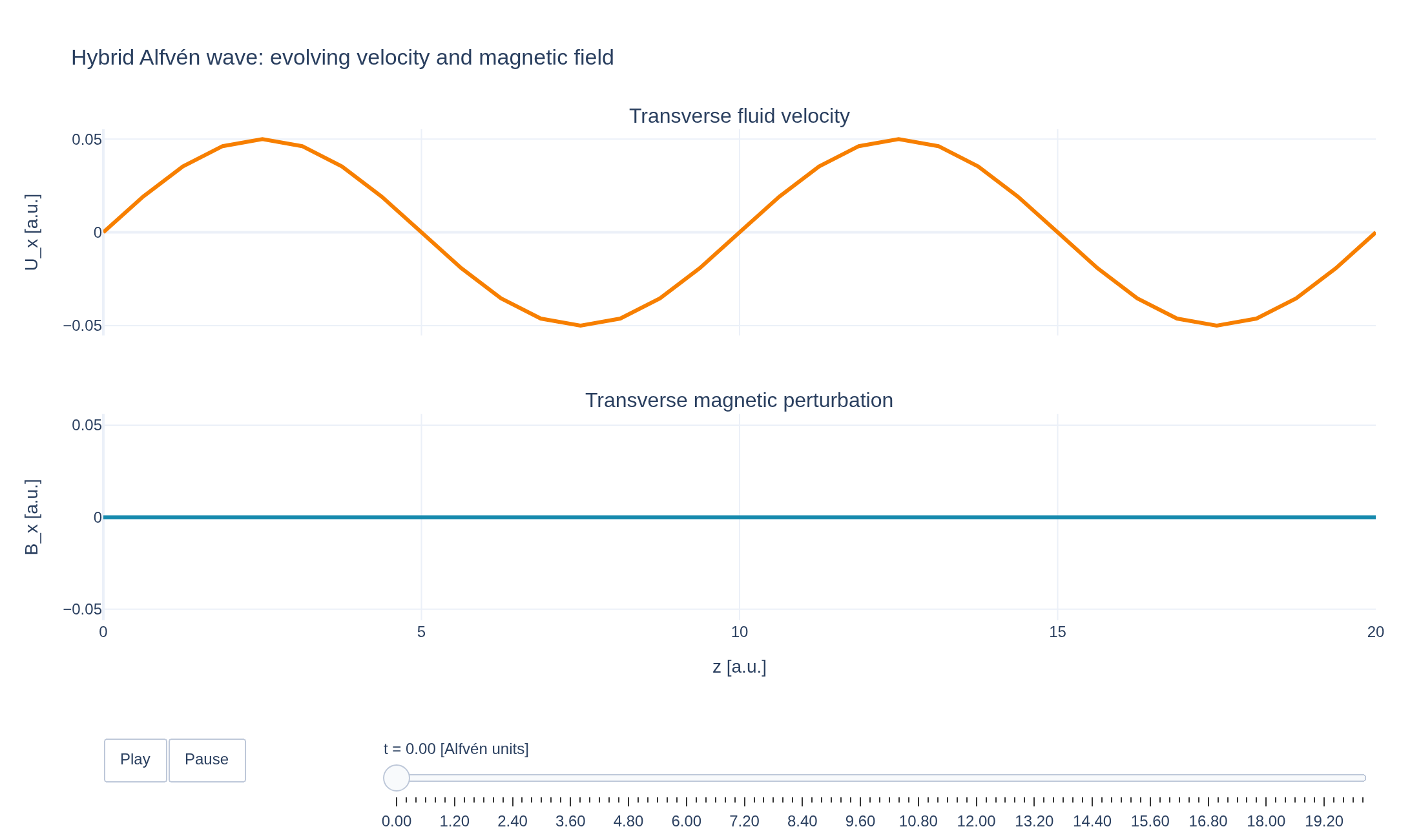
Loading interactive figure…
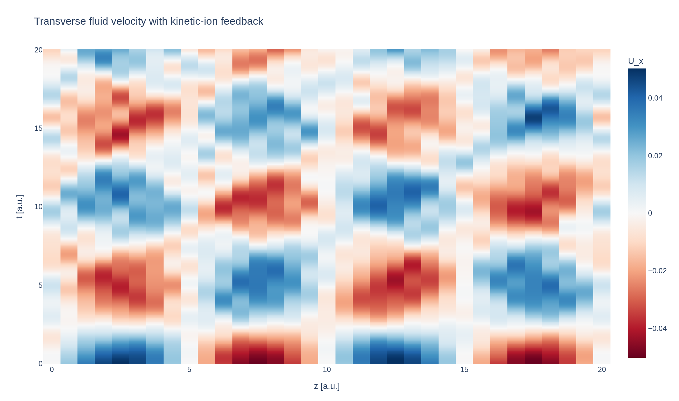
Loading interactive figure…
Physical problem
An Alfvén wave coupled to full-orbit ions
PDEs solved by model:
MHD continuity:
MHD momentum:
MHD pressure:
MHD induction:
Energetic-particle Vlasov equation:
Energetic-particle moments:
where .
Simulation geometry
Domain used in this run
The actual Cuboid geometry reconstructed from this run's metadata. Switch between the 3D view and physical-coordinate slices.
Domain
Cuboid
Mapping
Loading Cuboid…
Parameters
| Parameter | Value | Description |
|---|---|---|
| Loading parameters… | ||
Performance
Profiling
Struphy's built-in scope-profiler instruments every propagator, pusher and solver call — these are the real per-call timings from the run above.
Durations
Gantt (rank 0)
Region statistics
| Region | Count | Avg (s) | Min (s) | Max (s) | Total (s) |
|---|
Complete source
Simulation script
Requires Struphy with compiled kernels and Plotly. Run struphy compile once, then execute python hybrid-current-coupling.py.
"""An Alfvén wave coupled to kinetic ions with LinearMHDVlasovCC.

A transverse velocity mode perturbs a uniform MHD plasma. A dilute Maxwellian
population of energetic ions follows full particle orbits and feeds its current
back into the fluid momentum equation. The wave and the ions exchange energy
through the current-coupling scheme.

The energy plot subtracts the initial particle energy so that the exchange is
visible beside the much smaller wave energy. A separate diagnostic measures
total-energy error relative to the initial wave energy, including the pressure
channel. Finite marker sampling introduces noise; this is a coupling and
conservation demonstration, not a measurement of a kinetic damping rate.

Requires the repository's pinned Struphy with compiled kernels (`struphy compile`).
"""

import numpy as np

from struphy import (
    BoundaryParameters,
    DerhamOptions,
    EnvironmentOptions,
    LoadingParameters,
    SavingParameters,
    Simulation,
    SortingParameters,
    Time,
    WeightsParameters,
    domains,
    equils,
    grids,
    maxwellians,
    perturbations,
)
from struphy.linear_algebra.solver import SolverParameters
from struphy.models import LinearMHDVlasovCC

stem = "hybrid-current-coupling"
length = 20.0
amplitude = 0.05

# B0 = n0 = 1 sets v_A = 1; epsilon = 1 sets the hot-ion gyrofrequency.
model = LinearMHDVlasovCC(hot_epsilon=1.0)
# Resolve the small wave-energy exchange accurately against the ion background.
for propagator in (
    model.propagators.couple_dens, model.propagators.shear_alf,
    model.propagators.couple_curr, model.propagators.mag_sonic,
):
    propagator.options = propagator.Options(solver_params=SolverParameters(tol=1e-12))
model.mhd.velocity.save_data = True
model.em_fields.b_field.save_data = True
model.mhd.velocity.add_perturbation(
    perturbations.ModesSin(
        ns=(2,), amps=(amplitude,), comp=0, Lz=length, given_in_basis="physical",
    ),
)
model.energetic_ions.set_markers(
    loading_params=LoadingParameters(Np=8192, seed=7),
    weights_params=WeightsParameters(),
    boundary_params=BoundaryParameters(),
    sorting_params=SortingParameters(boxes_per_dim=(1, 1, 16), do_sort=True),
    saving_params=SavingParameters(),
)
model.energetic_ions.var.add_background(
    maxwellians.Maxwellian3D(
        n=(0.1, None), vth1=(0.5, None), vth2=(0.5, None), vth3=(0.5, None),
    ),
)

domain = domains.Cuboid(r3=length)
equil = equils.HomogenSlab(B0x=0.0, B0y=0.0, B0z=1.0, n0=1.0, beta=0.1)
grid = grids.TensorProductGrid(num_elements=(1, 1, 32))
derham_opts = DerhamOptions(degree=(1, 1, 3))
time_opts = Time(dt=0.05, Tend=20.0, split_algo="Strang")
env = EnvironmentOptions(out_folders="struphy_gallery_runs", sim_folder="hybrid_current_coupling")
sim = Simulation(
    model=model,
    name="Alfvén wave with kinetic-ion current coupling",
    description=(
        "A shear-Alfvén wave exchanges energy with a dilute population of kinetic ions. "
        "The LinearMHDVlasovCC hybrid model evolves the bulk plasma as a fluid and the "
        "energetic ions as particles, coupled through their current. Follow the wave "
        "and compare energy transfer with the total-energy conservation error."
        r" The fluid starts with $$u_x(z,0)=0.05\sin(\pi z/5),$$"
        r" in :math:`\mathbf{B}_0=\mathbf{e}_z`, :math:`n_0=1`. The energetic-ion Maxwellian has :math:`n_h=0.1`, :math:`\mathbf{u}_h=0` and isotropic thermal speed :math:`v_{\mathrm{th},h}=0.5`."
    ),
    env=env,
    time_opts=time_opts,
    domain=domain,
    equil=equil,
    grid=grid,
    derham_opts=derham_opts,
)


if __name__ == "__main__":
    import plotly.graph_objects as go
    from plotly.subplots import make_subplots

    from _gallery import export_profiling, is_root, merge_metadata, save_extra_figure, save_figure, space_time_figure

    output = sim.run(profiling_activated=True)
    output.pproc(physical=True)

    energies = {key: output.evaluate(key) for key in ("en_U", "en_B", "en_p", "en_f", "en_tot")}
    times = energies["en_tot"].t.values
    values = {key: data.values for key, data in energies.items()}
    if not all(np.isfinite(data).all() for data in values.values()):
        raise RuntimeError("The hybrid run produced non-finite energies")
    if not np.isclose(times[-1], time_opts.Tend):
        raise RuntimeError(f"The hybrid run stopped at t={times[-1]}, before t={time_opts.Tend}")
    if np.any(output.evaluate("n_lost_particles").values != 0):
        raise RuntimeError("Particles were lost from the periodic domain")
    velocity = output.evaluate("mhd/velocity_xyz").isel(e1=0, e2=0, component=0)
    if not np.isfinite(velocity.values).all():
        raise RuntimeError("The hybrid run produced a non-finite velocity field")
    magnetic = output.evaluate("em_fields/b_field_xyz").isel(e1=0, e2=0, component=0)
    if not np.isfinite(magnetic.values).all():
        raise RuntimeError("The hybrid run produced a non-finite magnetic field")
    if not np.array_equal(velocity.t.values, magnetic.t.values):
        raise RuntimeError("Velocity and magnetic snapshots must share the same times")

    wave_energy = float(values["en_U"][0] + values["en_B"][0])
    if wave_energy <= 0:
        raise RuntimeError("The initial wave energy must be positive")
    total_error = values["en_tot"] - values["en_tot"][0]
    relative_drift = float(np.max(np.abs(total_error)) / abs(values["en_tot"][0]))
    wave_scaled_error = float(np.max(np.abs(total_error)) / wave_energy)
    # Require conservation error below 0.1% of the seeded wave energy.
    # Plot the measured error explicitly; the run does not conserve to roundoff.
    if wave_scaled_error > 1e-3:
        raise RuntimeError(f"Total-energy error exceeds 0.1% of the initial wave energy: {wave_scaled_error:.2e}")
    if is_root():
        print(f"Maximum total-energy error / initial wave energy: {wave_scaled_error:.2e}")

    figure = make_subplots(
        rows=2, cols=1, shared_xaxes=True, vertical_spacing=0.17,
        subplot_titles=("Energy exchange", "Conservation error on the wave-energy scale"),
    )
    for key, label, color in (
        ("en_U", "MHD kinetic energy", "#f77f00"),
        ("en_B", "Magnetic energy", "#168aad"),
        ("en_f", "Ion energy change", "#d62828"),
        ("en_p", "Pressure energy change", "#6a4c93"),
    ):
        energy = values[key]
        if key in ("en_f", "en_p"):
            energy = energy - energy[0]
        figure.add_scatter(
            x=times, y=energy / wave_energy, mode="lines", name=label,
            line={"color": color, "width": 2.5}, row=1, col=1,
        )
    figure.add_scatter(
        x=times, y=1.0 + total_error / wave_energy, mode="lines", name="Sum of plotted channels",
        line={"color": "#222", "width": 1.5, "dash": "dash"}, row=1, col=1,
    )
    figure.add_scatter(
        x=times, y=total_error / wave_energy, mode="lines", name="Total-energy error",
        line={"color": "#222", "width": 2}, showlegend=False, row=2, col=1,
    )
    figure.update_yaxes(title_text="Energy / initial wave energy", row=1, col=1)
    figure.update_yaxes(title_text="ΔE_total / initial wave energy", row=2, col=1)
    figure.update_xaxes(title_text="t [Alfvén units]", row=2, col=1)
    figure.update_layout(
        title="Hybrid Alfvén wave: current coupling", template="plotly_white",
        legend={"orientation": "h", "y": -0.14},
        margin={"l": 85, "r": 35, "t": 100, "b": 130},
    )
    save_figure(figure, stem, height=800)

    # Animate physical field snapshots with fixed axes so amplitude changes remain visible.
    # Keep the first and last snapshots, with at most 101 frames for a compact download.
    frame_times = velocity.t.values
    picks = np.linspace(0, len(frame_times) - 1, min(101, len(frame_times)), dtype=int)

    def wave_traces(index):
        return [
            go.Scatter(
                x=field.e3.values * length, y=field.values[index], mode="lines",
                name=label, line={"color": color, "width": 3},
            )
            for field, label, color in (
                (velocity, "Fluid velocity U_x", "#f77f00"),
                (magnetic, "Magnetic perturbation B_x", "#168aad"),
            )
        ]

    animation = make_subplots(
        rows=2, cols=1, shared_xaxes=True, vertical_spacing=0.16,
        subplot_titles=("Transverse fluid velocity", "Transverse magnetic perturbation"),
    )
    for row, trace in enumerate(wave_traces(0), start=1):
        animation.add_trace(trace, row=row, col=1)
    animation.frames = [
        go.Frame(name=f"{frame_times[i]:.2f}", data=wave_traces(i), traces=[0, 1])
        for i in picks
    ]
    for row, field, label in ((1, velocity, "U_x [a.u.]"), (2, magnetic, "B_x [a.u.]")):
        limit = 1.1 * max(float(np.max(np.abs(field.values))), amplitude)
        animation.update_yaxes(title_text=label, range=[-limit, limit], row=row, col=1)
        animation.update_xaxes(range=[0, length], row=row, col=1)
    animation.update_xaxes(title_text="z [a.u.]", row=2, col=1)
    animation.update_layout(
        title="Hybrid Alfvén wave: evolving velocity and magnetic field",
        template="plotly_white", showlegend=False,
        margin={"l": 80, "r": 35, "t": 100, "b": 145},
        updatemenus=[{
            "type": "buttons", "showactive": False, "direction": "left",
            "x": 0, "xanchor": "left", "y": -0.24, "yanchor": "top",
            "buttons": [
                {"label": "Play", "method": "animate", "args": [None, {
                    "frame": {"duration": 70, "redraw": False},
                    "transition": {"duration": 0}, "fromcurrent": True,
                }]},
                {"label": "Pause", "method": "animate", "args": [[None], {
                    "mode": "immediate", "frame": {"duration": 0, "redraw": False},
                    "transition": {"duration": 0},
                }]},
            ],
        }],
        sliders=[{
            "active": 0, "x": 0.22, "len": 0.78, "y": -0.18,
            "currentvalue": {"prefix": "t = ", "suffix": " [Alfvén units]"},
            "steps": [
                {"label": frame.name, "method": "animate", "args": [[frame.name], {
                    "mode": "immediate", "frame": {"duration": 0, "redraw": False},
                    "transition": {"duration": 0},
                }]}
                for frame in animation.frames
            ],
        }],
    )
    figures = [save_extra_figure(
        animation, stem, "wave-animation",
        alt="Animated transverse velocity and magnetic perturbation along the periodic hybrid plasma slab",
        caption=(
            "Play or scrub through the wave evolution from t = 0 to 20. The upper panel shows the "
            "fluid velocity Uₓ and the lower panel the magnetic perturbation Bₓ, with fixed vertical "
            "scales to show their changing amplitudes as the wave exchanges energy with kinetic ions."
        ),
    )]

    wave = space_time_figure(
        velocity, space="e3", title="Transverse fluid velocity with kinetic-ion feedback",
        colorbar_title="U_x", xaxis_title="z [a.u.]", x_values=velocity.e3.values * length,
    )
    figures.append(save_extra_figure(
        wave, stem, "space-time",
        alt="Space-time map of the transverse MHD velocity coupled to kinetic ions",
        caption=(
            "The initial sinusoidal transverse velocity evolves in a periodic slab along B₀. "
            "Full-orbit ions feed their current back into the MHD wave; finite marker sampling adds noise."
        ),
    ))
    merge_metadata(
        stem,
        relativeTotalEnergyDrift=relative_drift,
        totalEnergyErrorOverInitialWaveEnergy=wave_scaled_error,
        initialWaveEnergy=wave_energy,
        figures=figures,
        **export_profiling(sim, stem),
    )
See the post-processing guide for more ways to inspect the result.