VariationalPressurelessFluid · Pressureless flow
Pressureless density transport
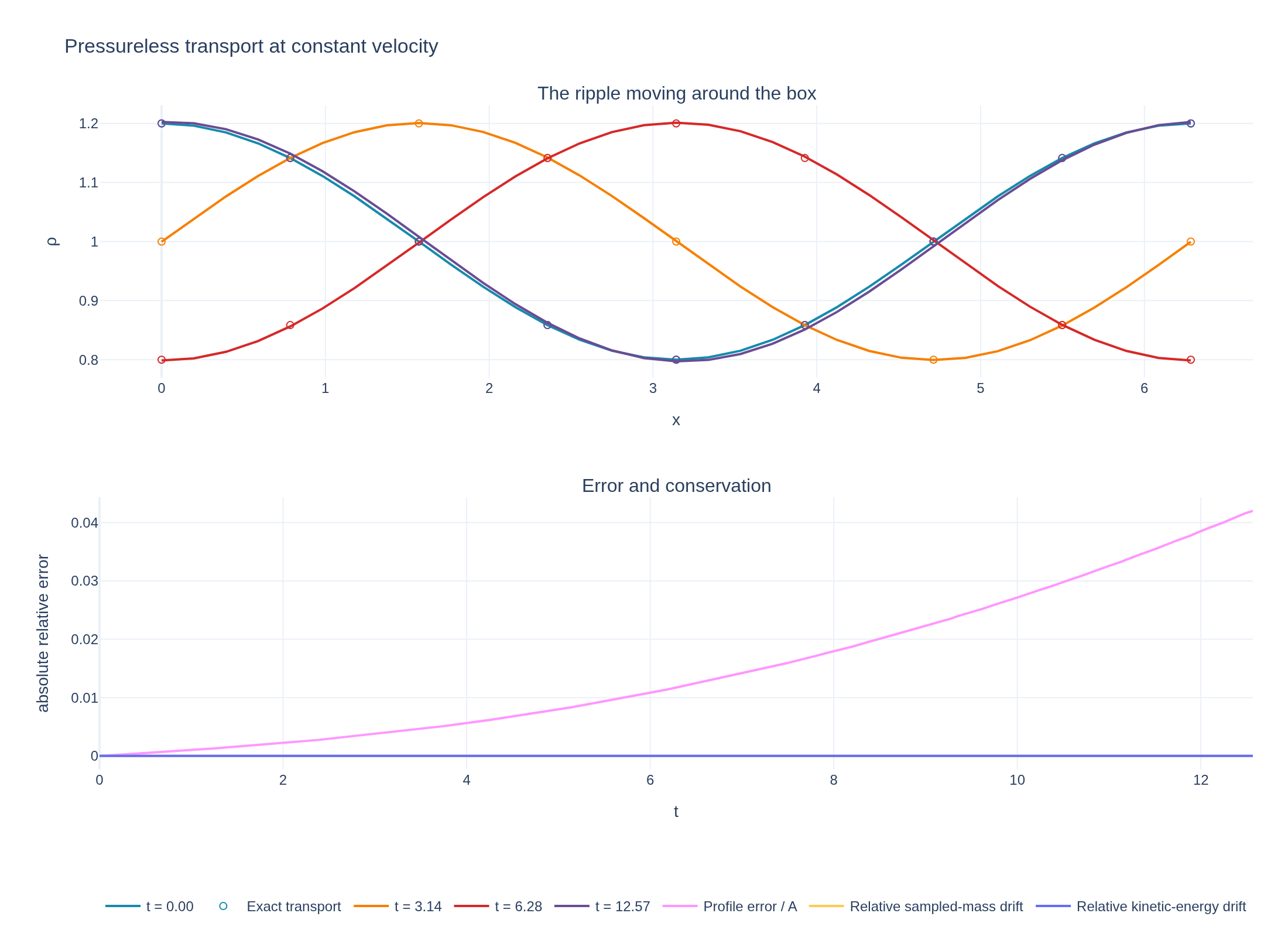
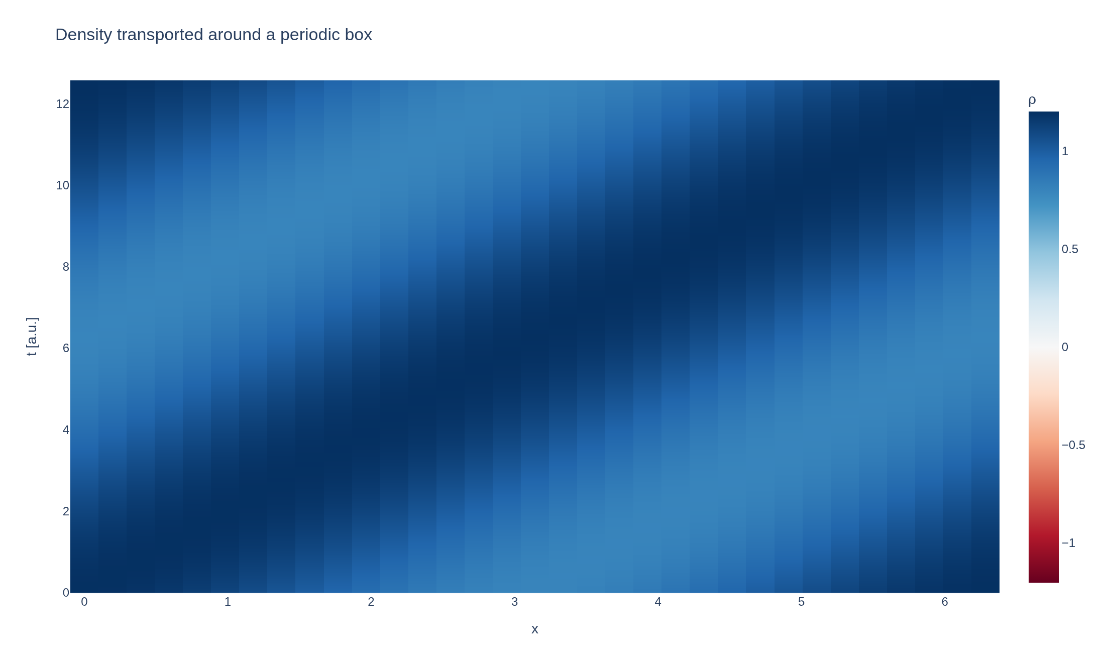
A density ripple travels once around a periodic box at constant speed. VariationalPressurelessFluid has no pressure force, so the exact nonlinear solution keeps the profile unchanged. Compare its shape, mass and kinetic energy. The initial data are giving on .
Loading interactive figure…
Loading interactive figure…
Physical problem
A density ripple carried at constant speed
PDEs solved by model:
Continuity:
Momentum:
Simulation geometry
Domain used in this run
The actual Cuboid geometry reconstructed from this run's metadata. Switch between the 3D view and physical-coordinate slices.
Domain
Cuboid
Mapping
Loading Cuboid…
Parameters
| Parameter | Value | Description |
|---|---|---|
| Loading parameters… | ||
Performance
Profiling
Struphy's built-in scope-profiler instruments every propagator, pusher and solver call — these are the real per-call timings from the run above.
Durations
Gantt (rank 0)
Region statistics
| Region | Count | Avg (s) | Min (s) | Max (s) | Total (s) |
|---|
Complete source
Simulation script
Requires Struphy with compiled kernels and Plotly. Run struphy compile once, then execute python pressureless-transport.py.
"""Exact density transport with VariationalPressurelessFluid.

Without pressure, a uniform velocity transports any smooth density profile
unchanged. Here rho = 1 + A cos(x - U t) makes one circuit of a periodic box.
This is an exact nonlinear solution, without characteristic crossing.

Requires the pinned Struphy with compiled kernels (`struphy compile`).
"""

import numpy as np

from struphy import (
    DerhamOptions, EnvironmentOptions, FieldsBackground, Simulation, Time,
    domains, equils, grids, perturbations,
)
from struphy.models import VariationalPressurelessFluid

stem = "pressureless-transport"
length, speed, amplitude = 2.0 * np.pi, 0.5, 0.2
crossing_time = length / speed
model = VariationalPressurelessFluid()
model.propagators.variat_dens.options = model.propagators.variat_dens.Options(model="pressureless")
# The density 3-form and contravariant velocity include the coordinate mapping.
model.fluid.density.add_background(FieldsBackground(values=(length,)))
model.fluid.velocity.add_background(FieldsBackground(values=(speed / length, 0.0, 0.0)))
model.fluid.density.add_perturbation(
    perturbations.ModesCos(ls=(1,), amps=(amplitude,), Lx=length, given_in_basis="physical"),
)
model.fluid.density.save_data = True
model.fluid.velocity.save_data = True
domain = domains.Cuboid(r1=length)
grid = grids.TensorProductGrid(num_elements=(32, 1, 1))
derham_opts = DerhamOptions(degree=(3, 1, 1))
time_opts = Time(dt=crossing_time / 800, Tend=crossing_time, split_algo="Strang")
sim = Simulation(
    model=model,
    name="Pressureless density transport",
    description=(
        "A density ripple travels once around a periodic box at constant speed. "
        "VariationalPressurelessFluid has no pressure force, so the exact nonlinear "
        "solution keeps the profile unchanged. Compare its shape, mass and kinetic energy."
        r" The initial data are $$\rho(x,0)=1+0.2\cos x,\qquad \mathbf{u}(x,0)=(0.5,0,0),$$"
        r" giving :math:`\rho(x,t)=1+0.2\cos(x-0.5t)` on :math:`0\leq x<2\pi`."
    ),
    env=EnvironmentOptions(out_folders="struphy_gallery_runs", sim_folder="pressureless_transport"),
    time_opts=time_opts, domain=domain, grid=grid, derham_opts=derham_opts,
    equil=equils.HomogenSlab(B0z=1.0, n0=1.0),
)


if __name__ == "__main__":
    from plotly.subplots import make_subplots

    from _gallery import export_profiling, merge_metadata, save_extra_figure, save_figure, space_time_figure

    output = sim.run(profiling_activated=True)
    output.pproc(physical=True)
    rho = output.evaluate("fluid/density_xyz").isel(e2=0, e3=0)
    velocity = output.evaluate("fluid/velocity_xyz").isel(component=0, e2=0, e3=0)
    energy = output.evaluate("kinetic_energy")
    times, x, density = rho.t.values, rho.e1.values * length, rho.values
    exact = 1.0 + amplitude * np.cos(x[None, :] - speed * times[:, None])
    if not all(np.isfinite(a).all() for a in (density, velocity.values, energy.values)):
        raise RuntimeError("The transport run produced non-finite diagnostics")
    if not np.isclose(times[-1], time_opts.Tend) or np.min(density) <= 0:
        raise RuntimeError("The transport run is incomplete or has non-positive density")
    errors = np.max(np.abs(density - exact), axis=1) / amplitude
    velocity_error = float(np.max(np.abs(velocity.values - speed)) / speed)
    energy_drift = float(np.max(np.abs(energy.values / energy.values[0] - 1.0)))
    # Sampled mass uses the periodic evaluation grid, dropping its repeated endpoint.
    mass = length * np.mean(density[:, :-1], axis=1)
    mass_drift = float(np.max(np.abs(mass / mass[0] - 1.0)))
    if errors.max() > 0.05 or velocity_error > 0.01 or max(energy_drift, mass_drift) > 1e-3:
        raise RuntimeError("Pressureless transport failed its profile or conservation checks")

    figure = make_subplots(rows=2, cols=1, vertical_spacing=0.18,
                           subplot_titles=("The ripple moving around the box", "Error and conservation"))
    for fraction, color in ((0.0, "#168aad"), (0.25, "#f77f00"), (0.5, "#d62828"), (1.0, "#6a4c93")):
        i = int(np.argmin(np.abs(times - fraction * crossing_time)))
        figure.add_scatter(x=x, y=density[i], name=f"t = {times[i]:.2f}", line={"color": color}, row=1, col=1)
        figure.add_scatter(x=x[::4], y=exact[i, ::4], mode="markers", name="Exact transport",
                           showlegend=fraction == 0.0, marker={"color": color, "symbol": "circle-open"}, row=1, col=1)
    for t, values, label in ((times, errors, "Profile error / A"),
                              (times, np.abs(mass / mass[0] - 1.0), "Relative sampled-mass drift"),
                              (energy.t.values, np.abs(energy.values / energy.values[0] - 1.0), "Relative kinetic-energy drift")):
        figure.add_scatter(x=t, y=values, name=label, row=2, col=1)
    figure.update_xaxes(title_text="x", row=1, col=1)
    figure.update_yaxes(title_text="ρ", row=1, col=1)
    figure.update_xaxes(title_text="t", row=2, col=1)
    figure.update_yaxes(title_text="absolute relative error", row=2, col=1)
    figure.update_layout(title="Pressureless transport at constant velocity", template="plotly_white",
                         legend={"orientation": "h", "y": -0.18}, margin={"l": 85, "r": 30, "t": 90, "b": 140})
    save_figure(figure, stem, height=800)
    movie = space_time_figure(rho, space="e1", x_values=x, xaxis_title="x",
                              title="Density transported around a periodic box", colorbar_title="ρ")
    figures = [save_extra_figure(movie, stem, "space-time", alt="Density ripple translating at constant speed",
                                caption="The diagonal bands travel at speed 0.5 and wrap through the periodic boundary.")]
    merge_metadata(stem, maxRelativeProfileError=float(errors.max()), maxRelativeVelocityError=velocity_error,
                   maxEnergyDrift=energy_drift, maxSampledMassDrift=mass_drift,
                   figures=figures, **export_profiling(sim, stem))
See the post-processing guide for more ways to inspect the result.