LinearMHD · MHD waves
Toroidal shear-Alfvén waves
A local preview of coupled poloidal shear-Alfvén perturbations in a circular tokamak, evolved with LinearMHD, including its magnetosonic propagator. The hollow torus has , major radius , and a periodic one-sixth toroidal sector. The AdhocTorus equilibrium uses , , and . The initial logical velocity combines , sector modes with amplitude parameter and Gaussian profiles centered at with width ; the poloidal component uses their radial derivatives. The coarse grid and short duration are intended for exploration, not a converged TAE benchmark. Plots show physical minor-radial, poloidal and toroidal velocity on the φ=0 slice; each component keeps its own fixed color range throughout the animation.
Loading interactive figure…
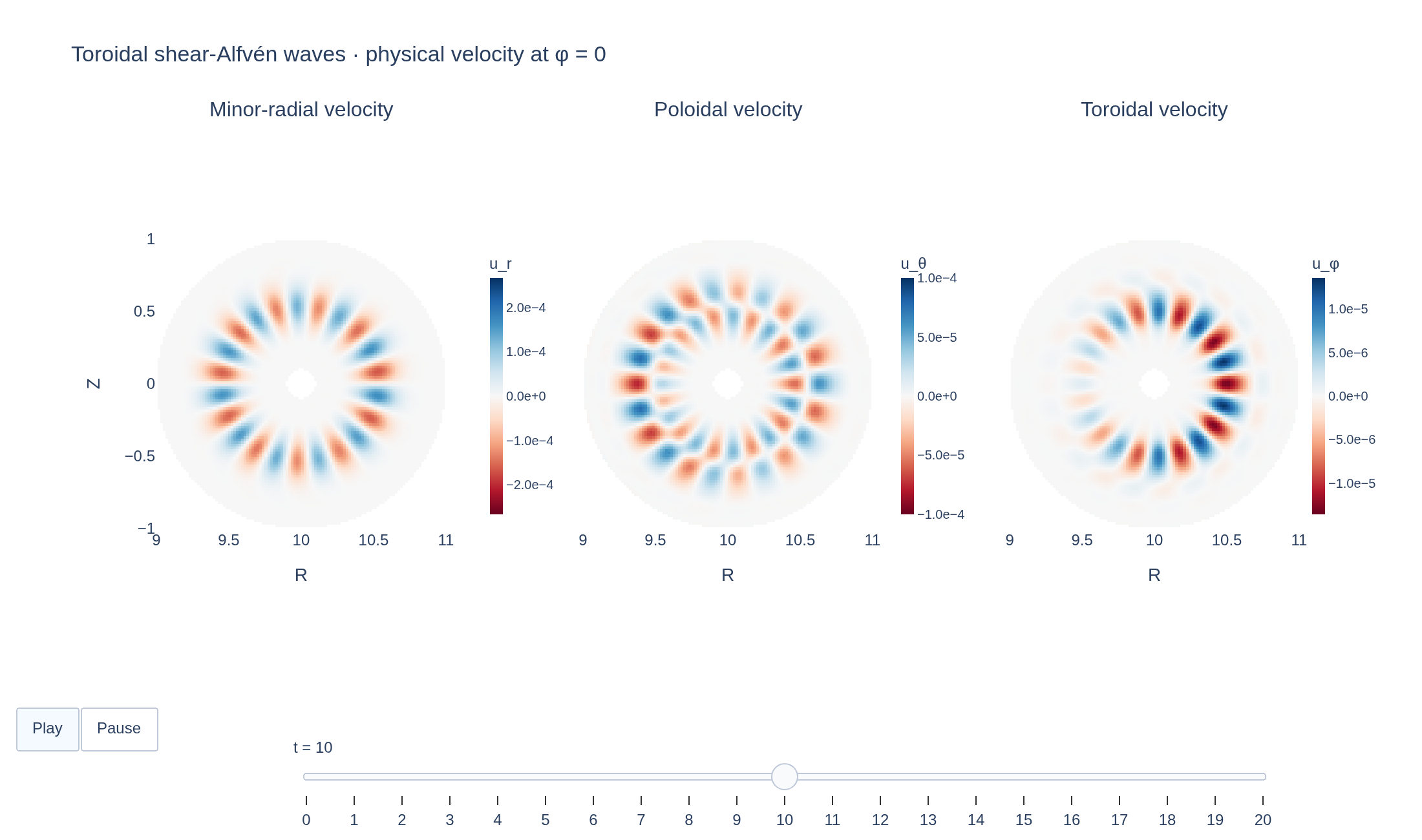
Loading interactive figure…
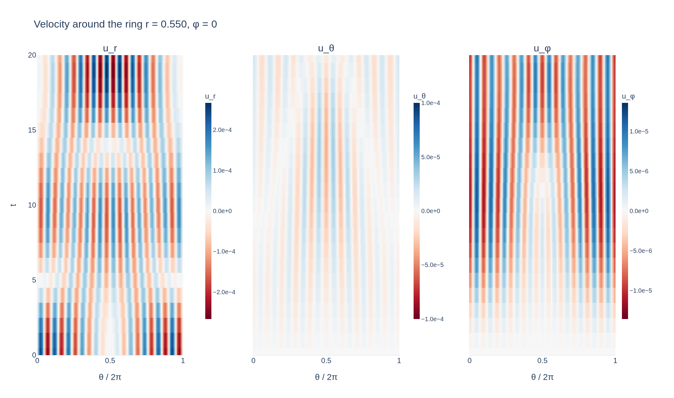
Loading interactive figure…
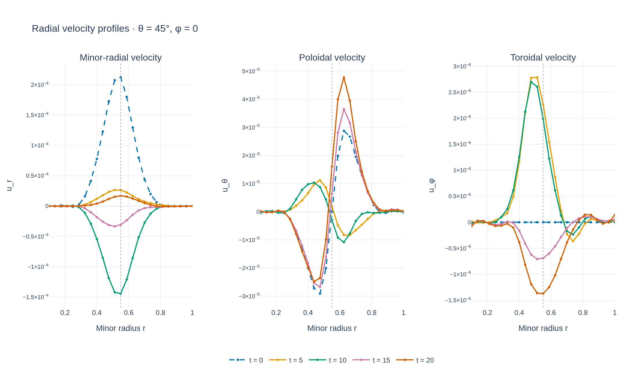
Loading interactive figure…
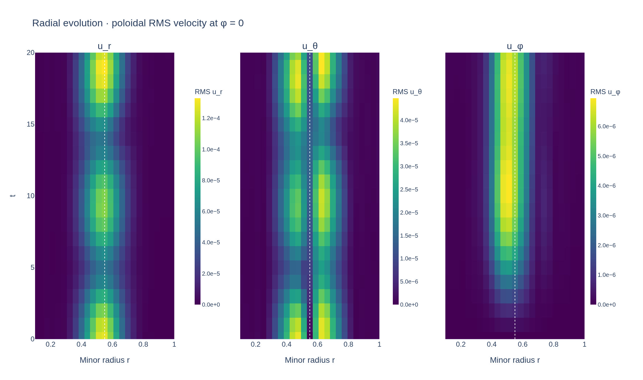
Loading interactive figure…
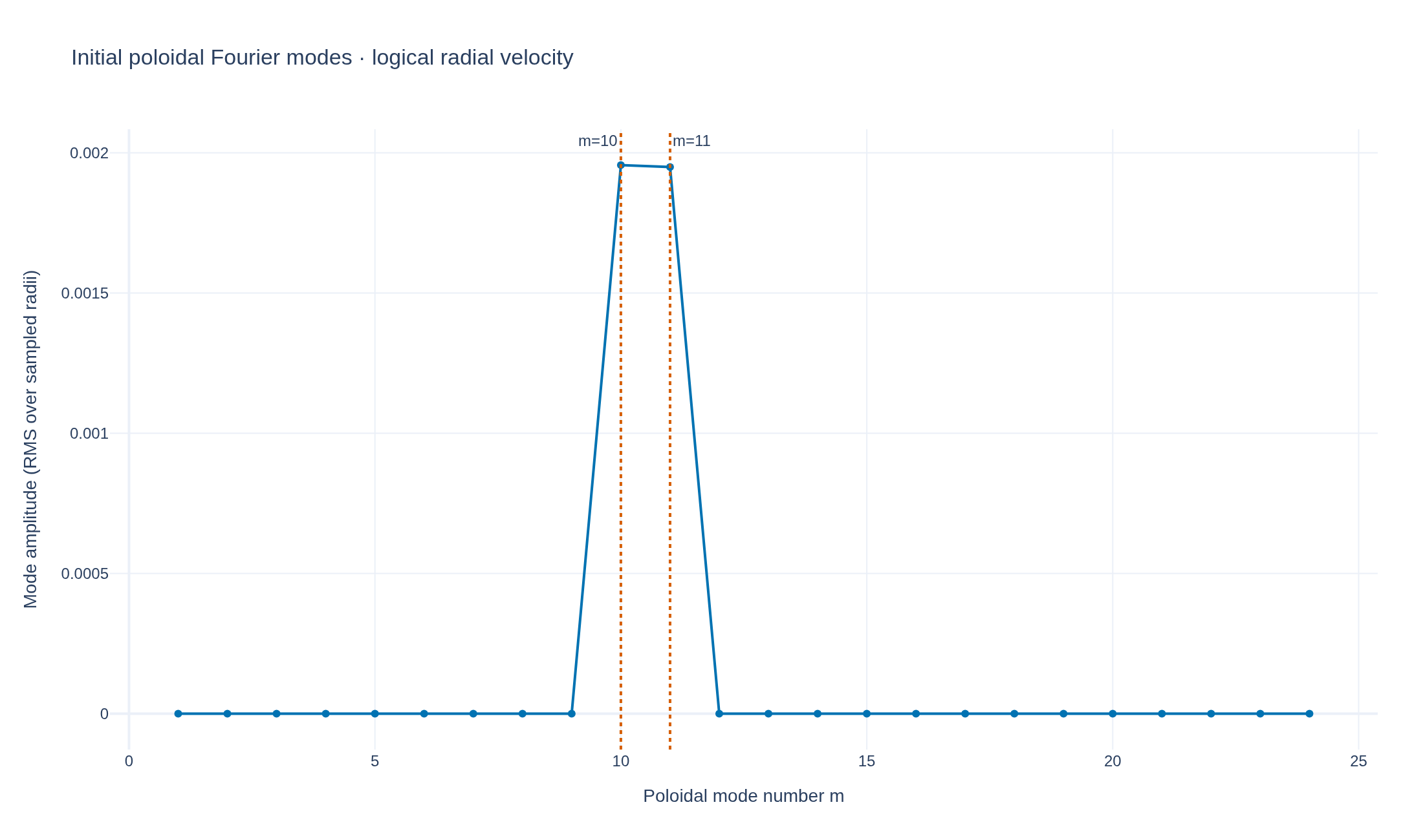
Loading interactive figure…
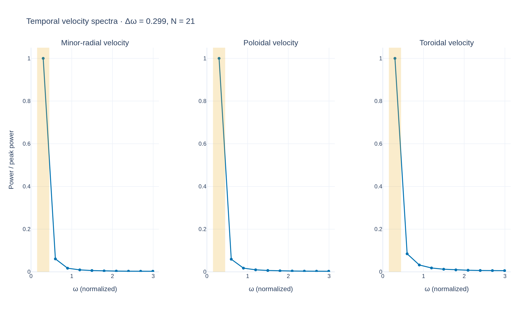
Loading interactive figure…
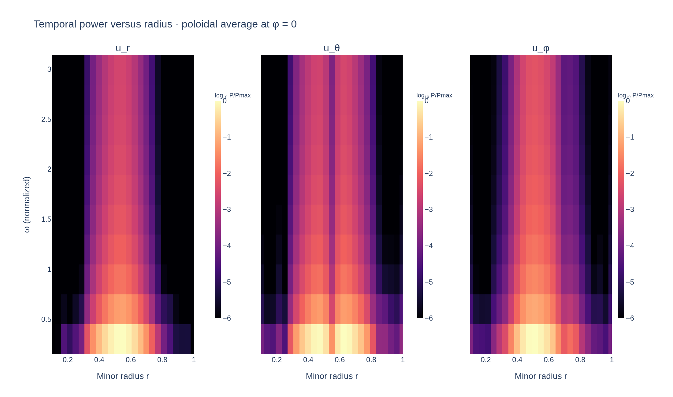
Loading interactive figure…
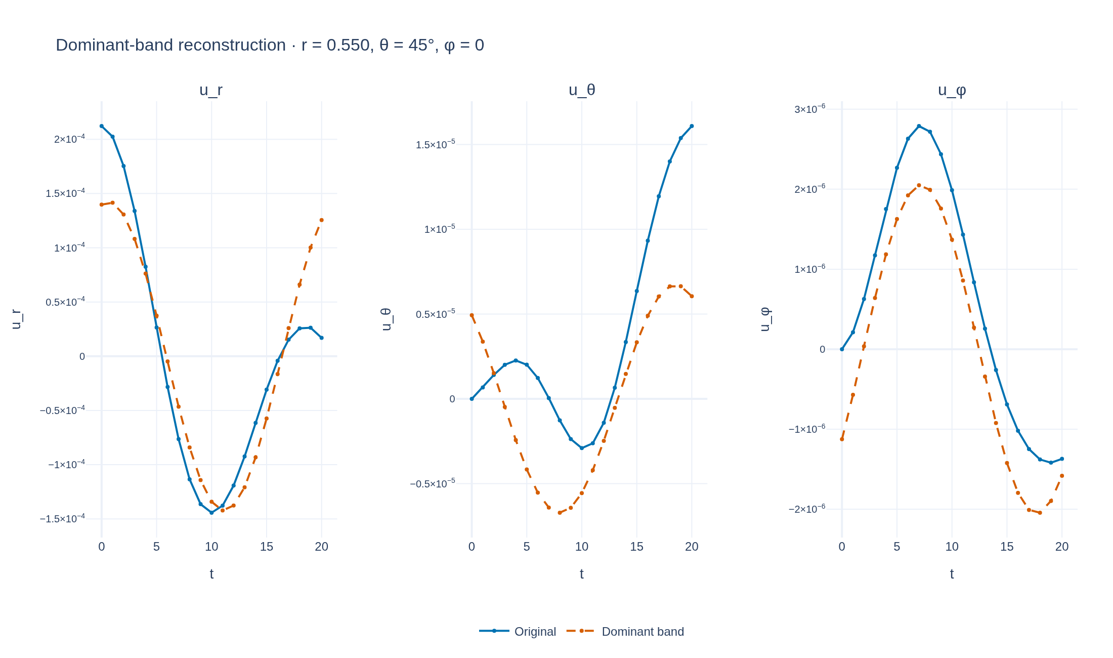
Loading interactive figure…
Physical problem
Coupled poloidal modes in a circular tokamak
PDEs solved by model:
Continuity (mass conservation):
Momentum (Lorentz force):
Energy (adiabatic process):
Induction (Faraday's law):
Simulation geometry
Domain used in this run
The actual HollowTorus geometry reconstructed from this run's metadata. Switch between the 3D view and physical-coordinate slices.
Domain
HollowTorus
Mapping
Loading HollowTorus…
Parameters
| Parameter | Value | Description |
|---|---|---|
| Loading parameters… | ||
Performance
Profiling
Struphy's built-in scope-profiler instruments every propagator, pusher and solver call — these are the real per-call timings from the run above.
Durations
Gantt (rank 0)
Region statistics
| Region | Count | Avg (s) | Min (s) | Max (s) | Total (s) |
|---|
Complete source
Simulation script
Requires Struphy with compiled kernels and Plotly. Run struphy compile once, then execute python toroidal-shear-alfven.py.
"""A small toroidal LinearMHD run with the m=10,11 shear-Alfvén perturbation.

Run from the repository root with:
    .venv/bin/python cli.py run toroidal-shear-alfven

Requires compiled Struphy kernels and Plotly's PNG exporter (see README.md).
The default is an exploratory local run, not a converged ITPA TAE benchmark.
Increase NUM_ELEMENTS to (24, 96, 16), DEGREE to (3, 3, 3), and END_TIME
to 500.0 to recover the supplied spatial/time resolution. The equilibrium,
sector, mode numbers, Gaussian profiles and amplitudes are retained.
"""

from time import perf_counter

import numpy as np
import plotly.graph_objects as go
from plotly.subplots import make_subplots
from scipy.ndimage import map_coordinates

from struphy import (
    BaseUnits,
    DerhamOptions,
    EnvironmentOptions,
    Simulation,
    Time,
    domains,
    equils,
    grids,
    perturbations,
)
from struphy.models import LinearMHD

STEM = "toroidal-shear-alfven"
NUM_ELEMENTS = (8, 48, 4)
DEGREE = (3, 3, 2)
END_TIME = 20.0
DT = 0.5
SAVE_STEP = 2

model = LinearMHD(base_units=BaseUnits())
model.propagators.shear_alf.options = model.propagators.shear_alf.Options()
model.propagators.mag_sonic.options = model.propagators.mag_sonic.Options()
for field in (model.em_fields.b_field, model.mhd.density, model.mhd.velocity, model.mhd.pressure):
    field.save_data = True

domain = domains.HollowTorus(a1=0.1, a2=1.0, R0=10.0, sfl=False, pol_period=1, tor_period=6)
equil = equils.AdhocTorus(
    a=1.0, R0=10.0, B0=3.0, q_kind=0, p_kind=1,
    q0=1.71, q1=1.87, p1=0.95, p2=0.05, beta=0.0018,
)
grid = grids.TensorProductGrid(num_elements=NUM_ELEMENTS)
derham_opts = DerhamOptions(degree=DEGREE, bcs=(("dirichlet", "dirichlet"), None, None))

# These are logical H(div) / 2-form components, not physical unit-vector
# components. TorusModes uses phase 2*pi*(m*eta2 + n*eta3); n=-1 is one
# oscillation across the 1/6-torus sector, not a full-torus n=-1 mode.
modes = (10, 11)
amplitude = 1e-3
model.mhd.velocity.add_perturbation(perturbations.TorusModesSin(
    ms=modes, ns=(-1, -1), amps=(amplitude, amplitude),
    pfuns=("exp", "exp"), pfun_params=([0.5, 0.1], [0.5, 0.1]),
    comp=0, given_in_basis="2",
))
model.mhd.velocity.add_perturbation(perturbations.TorusModesCos(
    ms=modes, ns=(-1, -1), amps=tuple(amplitude / (2 * np.pi * m) for m in modes),
    pfuns=("d_exp", "d_exp"), pfun_params=([0.5, 0.1], [0.5, 0.1]),
    comp=1, given_in_basis="2",
))

env = EnvironmentOptions(
    out_folders="struphy_gallery_runs", sim_folder="toroidal_shear_alfven",
    save_step=SAVE_STEP,
)
time_opts = Time(dt=DT, Tend=END_TIME)
sim = Simulation(
    model=model,
    name="Toroidal shear-Alfvén waves",
    description=(
        "A local preview of coupled poloidal shear-Alfvén perturbations in a circular tokamak, "
        "evolved with LinearMHD, including its magnetosonic propagator. "
        r"The hollow torus has :math:`0.1\le r\le1`, major radius :math:`R_0=10`, "
        r"and a periodic one-sixth toroidal sector. The AdhocTorus equilibrium uses "
        r":math:`B_0=3`, :math:`q_0=1.71`, :math:`q_1=1.87` and :math:`\beta=0.0018`. "
        r"The initial logical velocity combines :math:`m=10,11`, :math:`n=-1` sector modes "
        r"with amplitude parameter :math:`10^{-3}` and Gaussian profiles centered at "
        r":math:`\eta_1=0.5` with width :math:`0.1`; the poloidal component uses their radial derivatives. "
        "The coarse grid and short duration are intended for exploration, not a converged TAE benchmark. "
        "Plots show physical minor-radial, poloidal and toroidal velocity on the φ=0 slice; "
        "each component keeps its own fixed color range throughout the animation."
    ),
    params_path=__file__, env=env, time_opts=time_opts,
    domain=domain, equil=equil, grid=grid, derham_opts=derham_opts,
)

def plot_results(output, simulation_seconds):
    """Export the gallery figures; also usable with an existing Struphy Output."""
    from _gallery import export_profiling, merge_metadata, save_extra_figure, save_figure

    started = perf_counter()
    # More samples improve the display of the spline, not the simulation resolution.
    output.pproc(physical=True, celldivide=(3, 3, 1), create_vtk=False)
    velocity = output.evaluate("mhd/velocity_xyz").isel(e3=0).transpose("t", "component", "e1", "e2")
    times = velocity.t.values
    if not np.isclose(times[-1], END_TIME):
        raise RuntimeError(f"Run stopped at t={times[-1]}, before requested t={END_TIME}.")
    if not np.isfinite(velocity.values).all():
        raise RuntimeError("Non-finite velocity: refusing to export the example.")

    # At phi=0: e_R=e_x, e_phi=e_y, e_Z=e_z. Rotate the Cartesian
    # push-forward into orthonormal minor-radial and poloidal directions.
    theta = 2 * np.pi * velocity.e2.values
    ux, uy, uz = (velocity.isel(component=c).values for c in range(3))
    components = np.stack((
        ux * np.cos(theta) + uz * np.sin(theta),
        -ux * np.sin(theta) + uz * np.cos(theta),
        uy,
    ), axis=1)
    labels = ("u_r", "u_θ", "u_φ")
    titles = ("Minor-radial velocity", "Poloidal velocity", "Toroidal velocity")
    limits = np.maximum(np.abs(components).max(axis=(0, 2, 3)), 1e-16)

    # Resample the evaluated annulus onto pixels in the physical (R,Z) plane.
    # Use the actual evaluation coordinates; close the periodic angular seam.
    axis = np.linspace(-domain.params["a2"], domain.params["a2"], 112)
    pixel_r, pixel_z = np.meshgrid(axis, axis)
    radius = np.hypot(pixel_r, pixel_z)
    angle = np.mod(np.arctan2(pixel_z, pixel_r), 2 * np.pi) / (2 * np.pi)
    outside = (radius < domain.params["a1"]) | (radius > domain.params["a2"])
    eta1 = (radius - domain.params["a1"]) / (domain.params["a2"] - domain.params["a1"])
    radial_index = np.interp(eta1, velocity.e1.values, np.arange(velocity.sizes["e1"]))
    periodic = velocity.e2.values < 1.0 - 1e-12
    angular_grid = np.append(velocity.e2.values[periodic], 1.0)
    angular_index = np.interp(angle, angular_grid, np.arange(len(angular_grid)))

    def traces(index):
        result = []
        for component, label in enumerate(labels):
            values = components[index, component][:, periodic]
            values = np.concatenate((values, values[:, :1]), axis=1)
            pixels = map_coordinates(values, [radial_index, angular_index], order=1, mode="nearest")
            pixels[outside] = np.nan
            result.append(go.Heatmap(
                x=axis + domain.params["R0"], y=axis, z=pixels.astype(np.float32),
                zmin=-limits[component], zmax=limits[component], colorscale="RdBu",
                colorbar={
                    "title": label, "x": (0.28, 0.64, 1.0)[component], "len": 0.55,
                    "thickness": 10, "tickformat": ".1e", "tickfont": {"size": 10},
                },
                hovertemplate=f"R=%{{x:.3f}}<br>Z=%{{y:.3f}}<br>{label}=%{{z:.3e}}<extra></extra>",
                xaxis=f"x{component + 1}" if component else "x",
                yaxis=f"y{component + 1}" if component else "y",
            ))
        return result

    figure = make_subplots(rows=1, cols=3, subplot_titles=titles, horizontal_spacing=0.12)
    for column, trace in enumerate(traces(0), 1):
        figure.add_trace(trace, row=1, col=column)
    frame_indices = np.unique(np.linspace(0, len(times) - 1, min(26, len(times)), dtype=int))
    figure.frames = [go.Frame(name=f"{times[i]:g}", data=traces(i), traces=[0, 1, 2]) for i in frame_indices]
    figure.update_xaxes(
        title_text="R", range=[domain.params["R0"] - domain.params["a2"], domain.params["R0"] + domain.params["a2"]],
        constrain="domain", showgrid=False, zeroline=False,
    )
    for column in range(1, 4):
        figure.update_yaxes(
            title_text="Z" if column == 1 else None, range=[-domain.params["a2"], domain.params["a2"]],
            constrain="domain", showticklabels=column == 1, showgrid=False, zeroline=False,
            scaleanchor="x" if column == 1 else f"x{column}", scaleratio=1, row=1, col=column,
        )
    figure.update_layout(
        title="Toroidal shear-Alfvén waves · physical velocity at φ = 0",
        template="plotly_white", autosize=True, margin={"l": 55, "r": 95, "t": 95, "b": 130},
        sliders=[{
            "active": 0, "x": 0.12, "len": 0.86, "y": -0.12,
            "currentvalue": {"prefix": "t = "},
            "steps": [{"label": f.name, "method": "animate", "args": [[f.name], {
                "mode": "immediate", "frame": {"duration": 0, "redraw": True}, "transition": {"duration": 0},
            }]} for f in figure.frames],
        }],
        updatemenus=[{"type": "buttons", "direction": "left", "x": 0, "y": -0.12, "buttons": [
            {"label": "Play", "method": "animate", "args": [None, {
                "fromcurrent": True, "frame": {"duration": 100, "redraw": True}, "transition": {"duration": 0},
            }]},
            {"label": "Pause", "method": "animate", "args": [[None], {
                "mode": "immediate", "frame": {"duration": 0, "redraw": False},
            }]},
        ]}],
    )
    # A later snapshot also shows the generated toroidal component in the thumbnail.
    still = len(frame_indices) // 2
    save_figure(figure, STEM, static_data=traces(frame_indices[still]), static_active=still)

    radial_probe = int(np.abs(velocity.e1.values - 0.5).argmin())
    probe_radius = domain.params["a1"] + (domain.params["a2"] - domain.params["a1"]) * float(velocity.e1.values[radial_probe])
    history = make_subplots(rows=1, cols=3, subplot_titles=labels, horizontal_spacing=0.12)
    for component in range(3):
        history.add_trace(go.Heatmap(
            x=theta / (2 * np.pi), y=times, z=components[:, component, radial_probe],
            zmin=-limits[component], zmax=limits[component], colorscale="RdBu",
            colorbar={
                "title": labels[component], "x": (0.28, 0.64, 1.0)[component], "len": 0.8,
                "thickness": 10, "tickformat": ".1e", "tickfont": {"size": 10},
            },
        ), row=1, col=component + 1)
        history.update_yaxes(showticklabels=component == 0, range=[times[0], times[-1]], row=1, col=component + 1)
    history.update_xaxes(title_text="θ / 2π")
    history.update_yaxes(title_text="t", row=1, col=1)
    history.update_layout(
        title=f"Velocity around the ring r = {probe_radius:.3f}, φ = 0",
        template="plotly_white", margin={"l": 60, "r": 95, "t": 90, "b": 70},
    )

    # A radial ray away from the initial sine-mode node at theta=0. Select
    # an actual evaluation angle and report it, rather than relabeling it.
    radii = domain.params["a1"] + (domain.params["a2"] - domain.params["a1"]) * velocity.e1.values
    angle_probe = int(np.abs(theta - np.pi / 4).argmin())
    angle_degrees = float(np.degrees(theta[angle_probe]))
    initial_radius = domain.params["a1"] + 0.5 * (domain.params["a2"] - domain.params["a1"])
    snapshot_indices = np.unique(np.linspace(0, len(times) - 1, min(5, len(times)), dtype=int))
    snapshot_colors = ("#0072B2", "#E69F00", "#009E73", "#CC79A7", "#D55E00")
    radial_profiles = make_subplots(rows=1, cols=3, subplot_titles=titles, horizontal_spacing=0.12)
    for component, label in enumerate(labels):
        for snapshot, color in zip(snapshot_indices, snapshot_colors):
            radial_profiles.add_scatter(
                x=radii, y=components[snapshot, component, :, angle_probe],
                mode="lines+markers", name=f"t = {times[snapshot]:g}",
                legendgroup=str(snapshot), showlegend=component == 0,
                line={"color": color, "width": 2, "dash": "dash" if snapshot == 0 else "solid"},
                marker={"size": 4},
                hovertemplate=f"r=%{{x:.3f}}<br>{label}=%{{y:.3e}}<extra>t={times[snapshot]:g}</extra>",
                row=1, col=component + 1,
            )
        radial_profiles.update_yaxes(
            title_text=label, exponentformat="power", tickfont={"size": 10}, zeroline=True,
            row=1, col=component + 1,
        )
    radial_profiles.add_vline(x=initial_radius, line_dash="dot", line_color="#9ca3af", line_width=1)
    radial_profiles.update_xaxes(title_text="Minor radius r", range=[radii[0], radii[-1]])
    radial_profiles.update_layout(
        title=f"Radial velocity profiles · θ = {angle_degrees:g}°, φ = 0",
        template="plotly_white", margin={"l": 85, "r": 35, "t": 110, "b": 105},
        legend={"orientation": "h", "x": 0.5, "xanchor": "center", "y": -0.18},
    )

    # Angular RMS avoids cancellation between opposite signs of a wave.
    # Samples are uniform in theta; exclude the duplicate periodic endpoint.
    # This is an angular average on the phi=0 plane, not a volume average.
    angular_rms = np.sqrt(np.mean(components[..., periodic] ** 2, axis=-1))
    radial_history = make_subplots(rows=1, cols=3, subplot_titles=labels, horizontal_spacing=0.12)
    for component, label in enumerate(labels):
        radial_history.add_trace(go.Heatmap(
            x=radii, y=times, z=angular_rms[:, component],
            zmin=0, zmax=max(float(angular_rms[:, component].max()), 1e-16), colorscale="Viridis",
            colorbar={
                "title": f"RMS {label}", "x": (0.28, 0.64, 1.0)[component], "len": 0.8,
                "thickness": 10, "tickformat": ".1e", "tickfont": {"size": 10},
            },
            hovertemplate=f"r=%{{x:.3f}}<br>t=%{{y:g}}<br>RMS {label}=%{{z:.3e}}<extra></extra>",
        ), row=1, col=component + 1)
        radial_history.update_yaxes(
            showticklabels=component == 0, range=[times[0], times[-1]], row=1, col=component + 1,
        )
    radial_history.add_vline(x=initial_radius, line_dash="dot", line_color="white", line_width=1)
    radial_history.update_xaxes(title_text="Minor radius r", range=[radii[0], radii[-1]])
    radial_history.update_yaxes(title_text="t", row=1, col=1)
    radial_history.update_layout(
        title="Radial evolution · poloidal RMS velocity at φ = 0",
        template="plotly_white", margin={"l": 60, "r": 100, "t": 90, "b": 70},
    )

    # Transform signed physical components, before taking RMS or squaring:
    # transforming a velocity magnitude/energy would change its frequencies.
    # Omit the duplicated poloidal endpoint from spatial sums.
    plane = velocity.copy(data=components).assign_coords(component=list(labels))
    plane = plane.isel(e2=np.flatnonzero(periodic)).rename("physical_poloidal_velocity")
    temporal = output.time_fft(plane)
    band = output.filter_time(plane, dims=("e1", "e2"), pad_bins=0)
    positive = temporal.power.isel(omega=slice(1, None))
    omega = positive.omega.values
    frequency_resolution = temporal.attrs["frequency_resolution"]
    mean_power = positive.mean(("e1", "e2"))
    radius_power = positive.mean("e2")
    frequency_plot = make_subplots(rows=1, cols=3, subplot_titles=titles, horizontal_spacing=0.1)
    radius_spectrum = make_subplots(rows=1, cols=3, subplot_titles=labels, horizontal_spacing=0.12)
    filtered_probe = make_subplots(rows=1, cols=3, subplot_titles=labels, horizontal_spacing=0.12)
    for component, label in enumerate(labels):
        power = mean_power.isel(component=component).values
        frequency_plot.add_scatter(
            x=omega, y=power / max(float(power.max()), 1e-30), mode="lines+markers",
            name="Power", showlegend=False, line={"color": "#0072B2"}, row=1, col=component + 1,
        )
        selected = band.spectrum.isel(component=component)
        if bool(selected.has_peak):
            # Bin edges make a one-bin FWHM band visible; metadata retains bin centers.
            frequency_plot.add_vrect(
                x0=max(0, float(selected.omega_lo) - frequency_resolution / 2),
                x1=float(selected.omega_hi) + frequency_resolution / 2,
                fillcolor="#E69F00", opacity=0.2, line_width=0, row=1, col=component + 1,
            )
        local_power = radius_power.isel(component=component).transpose("omega", "e1").values
        log_power = np.log10(np.maximum(local_power / max(float(local_power.max()), 1e-30), 1e-6))
        radius_spectrum.add_trace(go.Heatmap(
            x=radii, y=omega, z=log_power, zmin=-6, zmax=0, colorscale="Magma",
            colorbar={"title": "log₁₀ P/Pmax", "x": (0.28, 0.64, 1.0)[component], "len": 0.8,
                      "thickness": 10, "title_font": {"size": 10}},
            hovertemplate="r=%{x:.3f}<br>ω=%{y:.3f}<br>log₁₀ P/Pmax=%{z:.2f}<extra></extra>",
        ), row=1, col=component + 1)
        radius_spectrum.update_yaxes(showticklabels=component == 0, row=1, col=component + 1)
        for field, name, color, dash in ((plane, "Original", "#0072B2", "solid"),
                                         (band.filtered, "Dominant band", "#D55E00", "dash")):
            probe = field.isel(component=component, e1=radial_probe, e2=angle_probe)
            filtered_probe.add_scatter(
                x=times, y=probe.values, mode="lines+markers", name=name, legendgroup=name,
                showlegend=component == 0, line={"color": color, "dash": dash}, marker={"size": 4},
                row=1, col=component + 1,
            )
        filtered_probe.update_yaxes(title_text=label, exponentformat="power", tickfont={"size": 10},
                                    row=1, col=component + 1)
    frequency_plot.update_xaxes(title_text="ω (normalized)", range=[0, temporal.attrs["nyquist_frequency"]])
    frequency_plot.update_yaxes(range=[0, 1.05])
    frequency_plot.update_yaxes(title_text="Power / peak power", row=1, col=1)
    frequency_plot.update_layout(
        title=f"Temporal velocity spectra · Δω = {frequency_resolution:.3f}, N = {len(times)}",
        template="plotly_white", margin={"l": 65, "r": 30, "t": 100, "b": 80},
    )
    radius_spectrum.update_xaxes(title_text="Minor radius r", range=[radii[0], radii[-1]])
    radius_spectrum.update_yaxes(title_text="ω (normalized)", row=1, col=1)
    radius_spectrum.update_layout(
        title="Temporal power versus radius · poloidal average at φ = 0",
        template="plotly_white", margin={"l": 85, "r": 100, "t": 90, "b": 70},
    )
    filtered_probe.update_xaxes(title_text="t")
    filtered_probe.update_layout(
        title=f"Dominant-band reconstruction · r = {probe_radius:.3f}, θ = {angle_degrees:g}°, φ = 0",
        template="plotly_white", margin={"l": 85, "r": 35, "t": 100, "b": 100},
        legend={"orientation": "h", "x": 0.5, "xanchor": "center", "y": -0.18},
    )

    # Check the seeded poloidal modes in the logical radial component, before
    # physical-basis rotation introduces additional geometric harmonics.
    logical_initial = output.evaluate("mhd/velocity").isel(t=0, component=0, e3=0)
    logical_initial = logical_initial.isel(e2=np.flatnonzero(periodic))
    poloidal_fft = output.fft(logical_initial, dim="e2")
    mode_numbers = poloidal_fft.k_e2.values / (2 * np.pi)
    modal_amplitude = np.sqrt((abs(poloidal_fft) ** 2).mean("e1")).values
    positive_modes = (mode_numbers > 0) & (mode_numbers <= grid.num_elements[1] // 2)
    mode_plot = go.Figure(go.Scatter(
        x=mode_numbers[positive_modes], y=2 * modal_amplitude[positive_modes], mode="lines+markers",
        line={"color": "#0072B2"}, name="Initial radial mode amplitude",
    ))
    for m in modes:
        mode_plot.add_vline(x=m, line_dash="dot", line_color="#D55E00", annotation_text=f"m={m}",
                            annotation_position="top left" if m == modes[0] else "top right")
    mode_plot.update_layout(
        title="Initial poloidal Fourier modes · logical radial velocity",
        xaxis_title="Poloidal mode number m", yaxis_title="Mode amplitude (RMS over sampled radii)",
        template="plotly_white", margin={"l": 85, "r": 35, "t": 100, "b": 70},
    )

    energy = go.Figure()
    for key, label in (("en_U", "Kinetic"), ("en_B", "Magnetic"), ("en_thermal", "Compressional")):
        values = output.evaluate(key)
        if not np.isfinite(values.values).all():
            raise RuntimeError(f"Non-finite energy diagnostic: {key}")
        energy.add_scatter(x=values.t.values, y=values.values, mode="lines", name=label)
    energy.update_layout(
        title="Perturbation energies", xaxis_title="t", yaxis_title="Energy [normalized units]",
        template="plotly_white", margin={"l": 80, "r": 30, "t": 80, "b": 65},
    )
    figures = [
        save_extra_figure(history, STEM, "velocity-history",
            alt="Time histories of three physical velocity components around a poloidal ring",
            caption=f"Physical velocity at r={probe_radius:.3f}, φ=0, over the complete run. "
            "The angular structure starts with the m=10,11 perturbations. Each panel uses the same "
            "component color range as the slice animation; interpolated display pixels do not add simulation resolution."),
        save_extra_figure(radial_profiles, STEM, "radial-profiles",
            alt="Radial profiles of three physical velocity components at five times",
            caption=f"Signed physical velocity along a radial ray at θ={angle_degrees:g}°, φ=0, "
            "from the inner to the outer boundary. Colors identify the same saved times in all three panels; "
            f"the dotted line marks the initial Gaussian center r={initial_radius:.3f}. "
            "Markers are spline evaluation points, not additional simulation cells. Velocities use normalized units."),
        save_extra_figure(radial_history, STEM, "radial-history",
            alt="Radius–time maps of the poloidal RMS of each physical velocity component",
            caption="The root-mean-square velocity over poloidal angle at each radius and time: "
            "sqrt(〈u²〉θ), evaluated on the φ=0 slice. This angular average shows radial localization "
            "without cancellation between positive and negative wave lobes; it is not a volume or flux-surface average. "
            "Each component has its own fixed color range in normalized velocity units. "
            f"The white dotted line marks the initial center r={initial_radius:.3f}; the underlying run still uses "
            f"only {grid.num_elements[0]} radial elements."),
        save_extra_figure(mode_plot, STEM, "poloidal-fft",
            alt="Initial logical radial velocity Fourier amplitudes with the seeded m=10 and m=11 modes",
            caption="Poloidal FFT of the initial logical H(div) radial velocity at φ=0. "
            "The duplicate periodic endpoint is excluded. Positive-mode amplitudes are 2|FFT|/N, "
            "followed by RMS over sampled radii, with no volume weighting. Dotted lines identify the seeded m=10,11 modes."),
        save_extra_figure(frequency_plot, STEM, "time-fft",
            alt="Temporal spectra of three physical velocity components with selected dominant frequency bands",
            caption="One-sided power per frequency bin from the signed velocity, averaged over sampled points "
            "in the φ=0 plane. DC is omitted and each panel is normalized to its own largest nonzero-frequency bin. "
            "Orange shading shows the contiguous half-power band used for reconstruction (no padding). "
            f"Saved spacing Δt={temporal.attrs['sample_spacing']:g}, N={len(times)}, Δω=2π/(NΔt)={frequency_resolution:.3f}, "
            f"and Nyquist frequency {temporal.attrs['nyquist_frequency']:.3f}. "
            "This short, untapered record has coarse frequency resolution and spectral leakage; its largest bin is not a converged TAE frequency."),
        save_extra_figure(radius_spectrum, STEM, "radial-time-fft",
            alt="Temporal velocity power as a function of minor radius and angular frequency",
            caption="Time FFT at each spatial point, followed by poloidal averaging of the power. "
            "Transforming the signed components before squaring avoids the frequency doubling of quadratic diagnostics. "
            "Colors show log₁₀(P/Pmax) separately for each component, clipped at −6; DC is omitted. "
            "The angular average is not weighted by physical volume. Only the actual frequency bins are displayed."),
        save_extra_figure(filtered_probe, STEM, "filtered-velocity",
            alt="Original and dominant-band-filtered velocity traces at a probe on the poloidal slice",
            caption=f"Original and reconstructed physical velocity at r={probe_radius:.3f}, θ={angle_degrees:g}°, φ=0. "
            "Each component's band is chosen from power summed over the whole sampled poloidal plane, then applied "
            "at every point before the inverse time FFT. DC and other bins are removed. "
            "This is a finite-record band-pass diagnostic, not an exact eigenmode; leakage and endpoint ringing remain possible."),
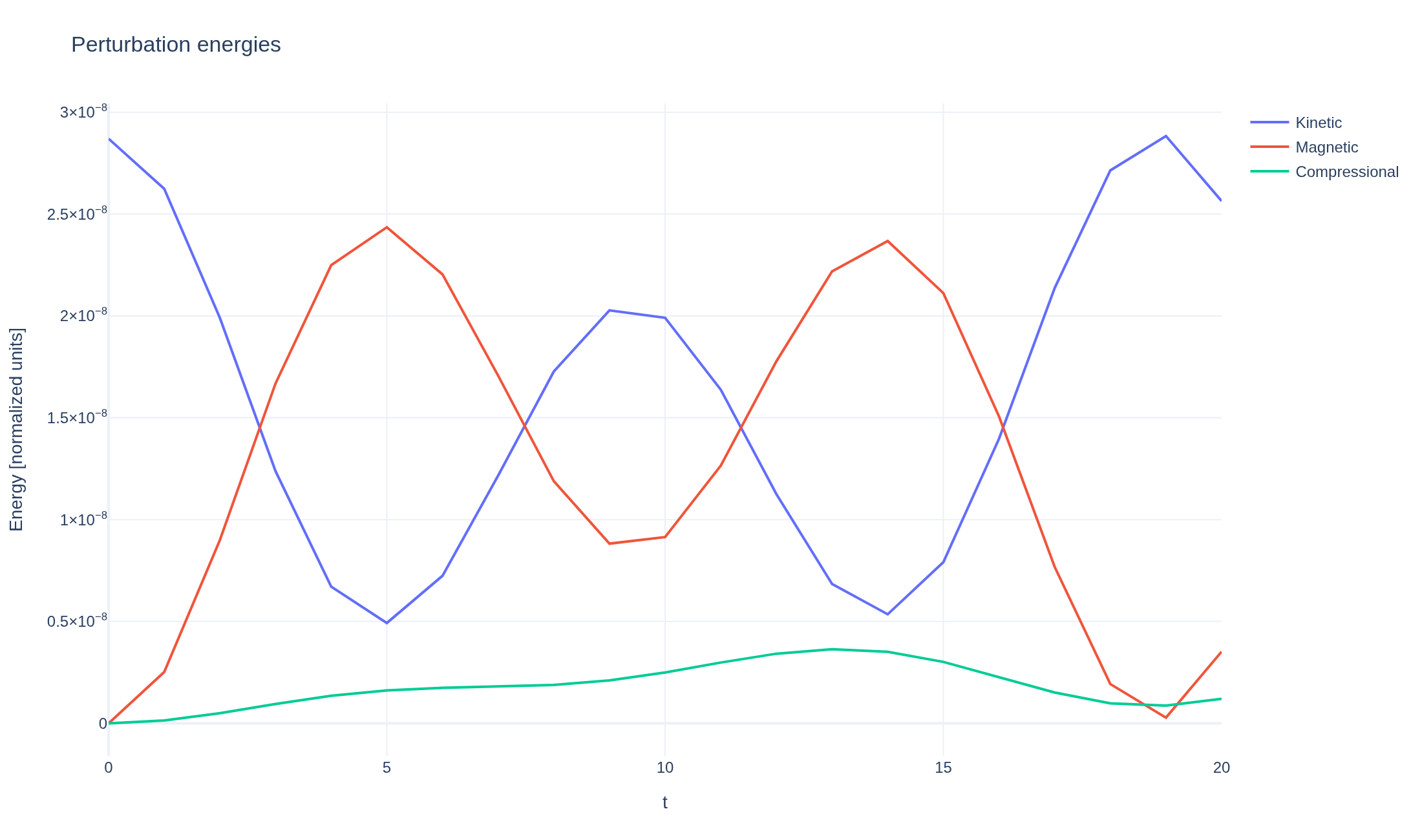
        save_extra_figure(energy, STEM, "energy",
            alt="Kinetic, magnetic and compressional perturbation energies over time",
            caption="Volume-integrated quadratic perturbation energies from LinearMHD. "
            "These exclude the equilibrium magnetic and thermal energies. They show the response of "
            "both the shear-Alfvén and magnetosonic propagators in the nonuniform toroidal equilibrium; "
            "this short coarse run does not establish a converged TAE frequency or growth rate."),
    ]
    merge_metadata(
        STEM, figures=figures, simulationSeconds=simulation_seconds,
        fftFrequencyResolution=frequency_resolution,
        fftDominantFrequencies=[float(value) if np.isfinite(value) else None
                               for value in band.spectrum.dominant_frequency.values],
        finalTime=float(times[-1]), savedFrames=len(times), **export_profiling(sim, STEM),
    )
    print(f"Simulation: {simulation_seconds:.1f} s; run and plots: {simulation_seconds + perf_counter() - started:.1f} s")


if __name__ == "__main__":
    started = perf_counter()
    output = sim.run(profiling_activated=True)
    plot_results(output, perf_counter() - started)
See the post-processing guide for more ways to inspect the result.